Probability distributions and Random Number Genereation
Probability distributions
To some extent, the foundation of statistics is an understanding of probability distributions. In addition, drawing of random samples from specific probability distributions is ubiquitous in applied statistics and useful in many contexts, not least of which is an appreciation of how different probabilty distriutions behave
help(Distributions)
| Distributions {stats} | R Documentation |
Distributions in the stats package
Description
Density, cumulative distribution function, quantile function and random variate generation for many standard probability distributions are available in the stats package.
Details
The functions for the density/mass function, cumulative distribution
function, quantile function and random variate generation are named in the
form dxxx, pxxx, qxxx and rxxx respectively.
For the beta distribution see dbeta.
For the binomial (including Bernoulli) distribution see
dbinom.
For the Cauchy distribution see dcauchy.
For the chi-squared distribution see dchisq.
For the exponential distribution see dexp.
For the F distribution see df.
For the gamma distribution see dgamma.
For the geometric distribution see dgeom. (This is also
a special case of the negative binomial.)
For the hypergeometric distribution see dhyper.
For the log-normal distribution see dlnorm.
For the multinomial distribution see dmultinom.
For the negative binomial distribution see dnbinom.
For the normal distribution see dnorm.
For the Poisson distribution see dpois.
For the Student's t distribution see dt.
For the uniform distribution see dunif.
For the Weibull distribution see dweibull.
For less common distributions of test statistics see
pbirthday, dsignrank,
ptukey and dwilcox (and see the
‘See Also’ section of cor.test).
See Also
RNG about random number generation in R.
The CRAN task view on distributions, http://cran.r-project.org/web/views/Distributions.html, mentioning several CRAN packages for additional distributions.
Basic functions for working with probabilty distributions —-
In the help documentaion, it is stated that “The functions for the density/mass function, cumulative distribution function, quantile function and random variate generation are named in the form dxxx, pxxx, qxxx and rxxx respectively”. We will explore what this means with a couple of examples.
Discrete distributions
For discrte distributions, the random values can only take integer values. One of the simplest discrete distributions is the Bernoulli distribution, where the only possible values are 0 (“Failure”) and 1 (“Success”). This has 2 parameters - the number of trials \(n\) and the probabilty of success in each trial \(p\). For example the Bernoulli distribution could model getting HEADs in a sequence or coin tosses, or whether a given subject in an experiment repsonds to a drug or not. Another discrete distribution is the Binomial distribution, which gives the probability of \(k\) successes in \(n\) trials. For example, the binomial distibution can tell you how many HEADS you get in 10 coin tosses for a biased coin wiht p=0.45. Note that the Bernoulli distribution can be considered a special case of the binomial distribution with a size of 1.
?rbinom
| Binomial {stats} | R Documentation |
The Binomial Distribution
Description
Density, distribution function, quantile function and random
generation for the binomial distribution with parameters size
and prob.
This is conventionally interpreted as the number of ‘successes’
in size trials.
Usage
dbinom(x, size, prob, log = FALSE)
pbinom(q, size, prob, lower.tail = TRUE, log.p = FALSE)
qbinom(p, size, prob, lower.tail = TRUE, log.p = FALSE)
rbinom(n, size, prob)
Arguments
x, q |
vector of quantiles. |
p |
vector of probabilities. |
n |
number of observations. If |
size |
number of trials (zero or more). |
prob |
probability of success on each trial. |
log, log.p |
logical; if TRUE, probabilities p are given as log(p). |
lower.tail |
logical; if TRUE (default), probabilities are P[X ≤ x], otherwise, P[X > x]. |
Details
The binomial distribution with size = n and
prob = p has density
p(x) = choose(n, x) p^x (1-p)^(n-x)
for x = 0, …, n.
Note that binomial coefficients can be computed by
choose in R.
If an element of x is not integer, the result of dbinom
is zero, with a warning.
is computed using Loader's algorithm, see the reference below.
The quantile is defined as the smallest value x such that F(x) ≥ p, where F is the distribution function.
Value
dbinom gives the density, pbinom gives the distribution
function, qbinom gives the quantile function and rbinom
generates random deviates.
If size is not an integer, NaN is returned.
The length of the result is determined by n for
rbinom, and is the maximum of the lengths of the
numerical arguments for the other functions.
The numerical arguments other than n are recycled to the
length of the result. Only the first elements of the logical
arguments are used.
Source
For dbinom a saddle-point expansion is used: see
Catherine Loader (2000). Fast and Accurate Computation of Binomial Probabilities; available from http://www.herine.net/stat/software/dbinom.html.
pbinom uses pbeta.
qbinom uses the Cornish–Fisher Expansion to include a skewness
correction to a normal approximation, followed by a search.
rbinom (for size < .Machine$integer.max) is based on
Kachitvichyanukul, V. and Schmeiser, B. W. (1988) Binomial random variate generation. Communications of the ACM, 31, 216–222.
For larger values it uses inversion.
See Also
Distributions for other standard distributions, including
dnbinom for the negative binomial, and
dpois for the Poisson distribution.
Examples
require(graphics)
# Compute P(45 < X < 55) for X Binomial(100,0.5)
sum(dbinom(46:54, 100, 0.5))

## Using "log = TRUE" for an extended range :
n <- 2000
k <- seq(0, n, by = 20)
plot (k, dbinom(k, n, pi/10, log = TRUE), type = "l", ylab = "log density",
      main = "dbinom(*, log=TRUE) is better than  log(dbinom(*))")
lines(k, log(dbinom(k, n, pi/10)), col = "red", lwd = 2)
## extreme points are omitted since dbinom gives 0.
mtext("dbinom(k, log=TRUE)", adj = 0)
mtext("extended range", adj = 0, line = -1, font = 4)
mtext("log(dbinom(k))", col = "red", adj = 1)
The rxxx family
If I coss a toin with probablity of heads = 0.45, how many heads do I see? Let’s simulate this experiemnt by drawing random numbers from the Bernoulli distribution (or equivalently the binomial distribution with size=1).
rbinom(n=100, prob=0.45, size=1)
- 1
- 0
- 1
- 1
- 1
- 0
- 0
- 1
- 1
- 0
- 0
- 1
- 0
- 1
- 1
- 0
- 0
- 0
- 0
- 0
- 0
- 1
- 0
- 0
- 1
- 0
- 1
- 0
- 0
- 0
- 0
- 1
- 0
- 1
- 1
- 0
- 1
- 0
- 0
- 1
- 0
- 1
- 0
- 1
- 1
- 0
- 0
- 1
- 0
- 0
- 1
- 1
- 0
- 1
- 0
- 1
- 1
- 0
- 1
- 1
- 1
- 1
- 0
- 0
- 0
- 0
- 0
- 1
- 1
- 0
- 0
- 0
- 0
- 0
- 0
- 1
- 0
- 1
- 1
- 0
- 0
- 1
- 0
- 1
- 0
- 1
- 0
- 1
- 0
- 0
- 1
- 1
- 1
- 0
- 1
- 0
- 0
- 0
- 1
- 0
How many heads do we see if we repeat this experiemnt 10 times?
rbinom(n=10, prob=0.45, size=100)
- 44
- 42
- 37
- 50
- 45
- 47
- 52
- 47
- 38
- 52
It should be clear that the number of heads we observe is alwayss a number between 0 and 100. What is the probabily of observing exactly 35 heades?
The dxxx family
dbinom(x=35, prob=0.45, size=100)
Let’s plot the proabbity for all numbers from 0 to 100.
plot(dbinom(x=0:100, prob=0.45, size=100))

The pxxx family
We can also see the cumulative probabilty of otbaiining a certain number
of heads with pbinom.
plot(pbinom(0:100, prob=0.45, size=100))

The qxxx family
The qxxx or quantile function is a little more tricky to understand.
One way to think about it is to look at the cumulative distirbution plot
and ask - If I start with a horizontal line from the y-axis at some
value p between 0 and 1 until I hit the funciton, then drop a veritcal
line to teh x-axis, what is the value I get? For example, what is the
number of heads where the cumulative distribution first reaches a value
of 0.5?
qbinom(p = 0.5, prob = 0.45, size=100)
Work!
What is the mean, median and standard deviation of the number of heads if the probabilty of heads is 0.4 and we toss 50 coins per experiment? Do 1000 such experiments and use the appropirate R functions to callculate these summary statistics.
What is the probability of getting between 2 to 5 (that is 2, 3, 4 or 5) sixes in 10 rolls of a fair six-sided die?
Explore what the Poisson distribution is (e.g. see Wikipedia and R help). Suppose there is on averate one mutation every 10,000 bases. What is the probabilty of finding exactly 8 mutations in 100,000 bases? What is the prrobability fo finding 15 or more mutations in 100,000 bases?
Continuous Distributions
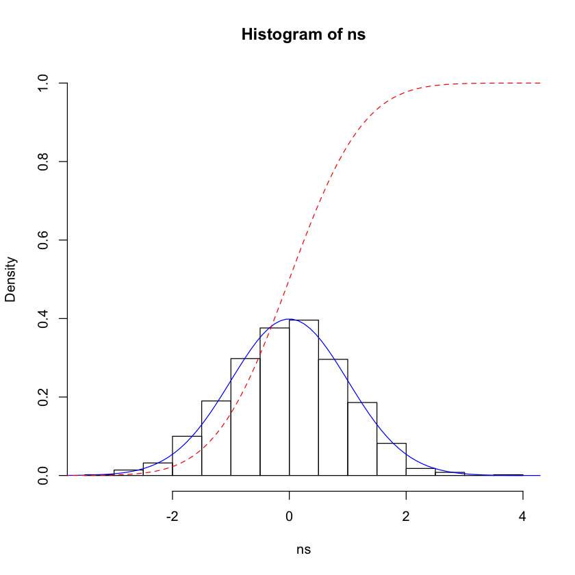
Distributions can also be continuous - a familiar example is the normal distribution.
x <- seq(-5, 5, length.out = 100)
ns <- rnorm(n=1000, mean=0.0, sd=1.0)
hist(ns, probability=TRUE, ylim = c(0, 1))
lines(x, dnorm(x), type="l", col="blue")
lines(x, pnorm(x), type="l", lty=2, col="red")
If IQ is normally distributed, the mean IQ is 100 with a standard deviation of 15, and you have an IQ of 135, what percentage of people have IQs higher than you?
Suppose that you toss 100 unbiased conis per experiemnt and count the number of heads. Plot the density function of this discrete distribution. Now superimpose a normal distribution density function with mean 50 and standard deviation of 5. What do you observe?