Unsupervised Learning¶

Preprocessing¶

When calculating distances, we usually want the features to be measured on thes same scale. One popular way of doing this is to transform each feature so that it has a mean of zero (centering) and a standard devaition of one (scaling).

x <- matrix(rnorm(20), nrow=5)
colnames(x) <- paste("Feature", 1:4)
rownames(x) <- paste("PDD", 1:5)
x <- matrix(rep(c(1,2,10,100), 5), nrow=5, byrow = TRUE) * x
x

       Feature 1 Feature 2 Feature 3 Feature 4
PDD 1 -0.6312717 1.3940762  12.62903 102.12761
PDD 2 -0.4718824 0.1974441  12.38225 229.10370
PDD 3  0.6633411 1.1548665  11.40228 -37.56147
PDD 4 -0.7970284 1.3718478  11.82333  80.73873
PDD 5  0.1236836 0.7267897 -24.07455 -85.34598

Pairwise distances¶

dist(x, method = "euclidean", upper = FALSE)

         PDD 1    PDD 2    PDD 3    PDD 4
PDD 2 126.9821
PDD 3 139.7007 266.6711
PDD 4  21.4047 148.3710 118.3102
PDD 5 191.0354 316.5570  59.5184 169.9237

Scaling¶

y <- scale(x, center = TRUE, scale = TRUE)
y

       Feature 1  Feature 2  Feature 3  Feature 4
PDD 1 -0.6754783  0.8370665  0.4822636  0.3576222
PDD 2 -0.4120093 -1.5193866  0.4669988  1.3823173
PDD 3  1.4645045  0.3660058  0.4063815 -0.7696667
PDD 4 -0.9494727  0.7932936  0.4324263  0.1850142
PDD 5  0.5724557 -0.4769793 -1.7880703 -1.1552870
attr(,"scaled:center")
 Feature 1  Feature 2  Feature 3  Feature 4
-0.2226316  0.9690049  4.8324703 57.8125180
attr(,"scaled:scale")
  Feature 1   Feature 2   Feature 3   Feature 4
  0.6049641   0.5078107  16.1666007 123.9159591

apply(y, MARGIN = 2, FUN = mean)

    Feature 1     Feature 2     Feature 3     Feature 4
-4.440892e-17  9.992007e-17 -2.220446e-17  3.332837e-17

apply(y, 2, sd)

Feature 1 Feature 2 Feature 3 Feature 4
        1         1         1         1

Pairwsie distances¶

dist(y)

          PDD 1     PDD 2     PDD 3     PDD 4
PDD 2 2.5831222
PDD 3 2.4653525 3.4220926
PDD 4 0.3305545 2.6593394 2.6309608
PDD 5 3.2752658 3.6851807 2.5437564 3.2644864

Dimension reduction¶

head(iris, 3)

  Sepal.Length Sepal.Width Petal.Length Petal.Width Species
        5.1         3.5          1.4         0.2  setosa
        4.9         3.0          1.4         0.2  setosa
        4.7         3.2          1.3         0.2  setosa

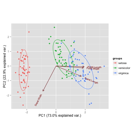
ir <- iris[,1:4]

ir.pca <- prcomp(ir,
                 center = TRUE,
                 scale. = TRUE)

summary(ir.pca)

Importance of components:
                          PC1    PC2     PC3     PC4
Standard deviation     1.7084 0.9560 0.38309 0.14393
Proportion of Variance 0.7296 0.2285 0.03669 0.00518
Cumulative Proportion  0.7296 0.9581 0.99482 1.00000

plot(ir.pca, type="l")

options(warn=-1)
suppressMessages(install.packages("devtools",repos = "http://cran.r-project.org"))
library(devtools)
suppressMessages(install_github("vqv/ggbiplot"))
library(ggbiplot)
options(warn=0)

The downloaded binary packages are in
    /var/folders/bh/x038t1s943qftp7jzrnkg1vm0000gn/T//RtmpYzgefV/downloaded_packages

Loading required package: ggplot2
Loading required package: plyr
Loading required package: scales
Loading required package: grid

ggbiplot(ir.pca, groups = iris$Species, var.scale=1, obs.scale=1, ellipse = TRUE)

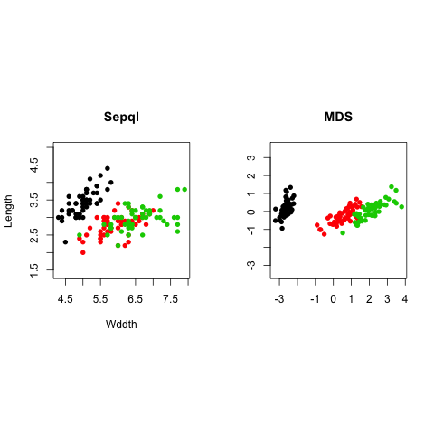
ir.mds <- cmdscale(dist(ir), k = 2)

par(mfrow=c(1,2), pty="s")
plot(iris[,1], iris[,2], type = "p", asp = 1, col=iris$Species, pch=16, main="Sepal", xlab="Wddth", ylab="Length")
plot(ir.mds[,1], ir.mds[,2], type = "p", asp = 1, col=iris$Species, pch=16, main="MDS", xlab="", ylab="")

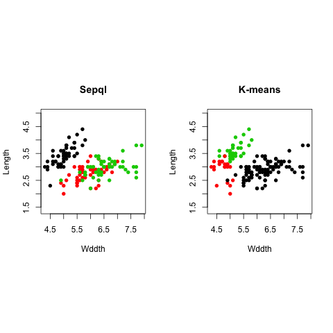
Clustering¶

ir.kmeans <- kmeans(ir, centers=3)

par(mfrow=c(1,2), pty="s")
plot(iris[,1], iris[,2], type = "p", asp = 1, col=iris$Species, pch=16, main="True", xlab="Wddth", ylab="Length")
plot(iris[,1], iris[,2], type = "p", asp = 1, col=ir.kmeans$cluster, pch=16,
     main="K-means", xlab="Wddth", ylab="Length")

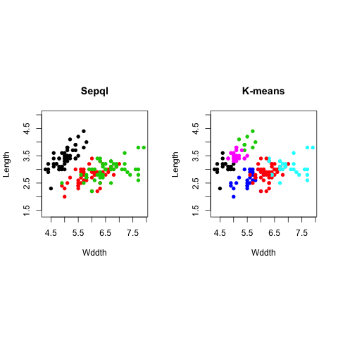
ir.kmeans <- kmeans(ir, centers=6)

par(mfrow=c(1,2), pty="s")
plot(iris[,1], iris[,2], type = "p", asp = 1, col=iris$Species, pch=16, main="True", xlab="Wddth", ylab="Length")
plot(iris[,1], iris[,2], type = "p", asp = 1, col=ir.kmeans$cluster, pch=16,
     main="K-means", xlab="Wddth", ylab="Length")

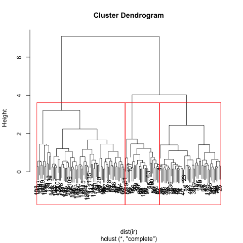
ir.ahc <- hclust(dist(ir), method = "complete")

plot(ir.ahc)
rect.hclust(ir.ahc, k=3, border = "red")

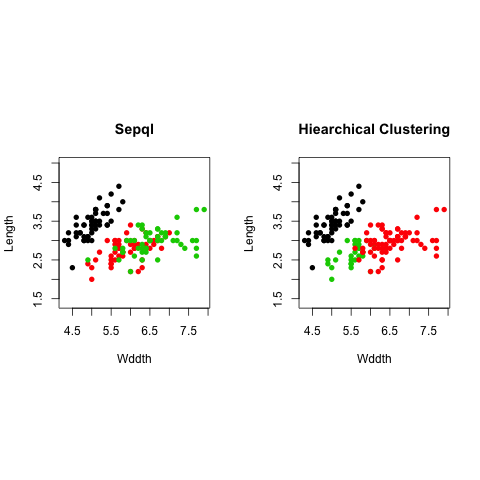
groups <- cutree(ir.ahc, k=3)

par(mfrow=c(1,2), pty="s")
plot(iris[,1], iris[,2], type = "p", asp = 1, col=iris$Species, pch=16, main="True", xlab="Wddth", ylab="Length")
plot(iris[,1], iris[,2], type = "p", asp = 1, col=groups, pch=16,
     main="Hiearchical Clustering", xlab="Wddth", ylab="Length")

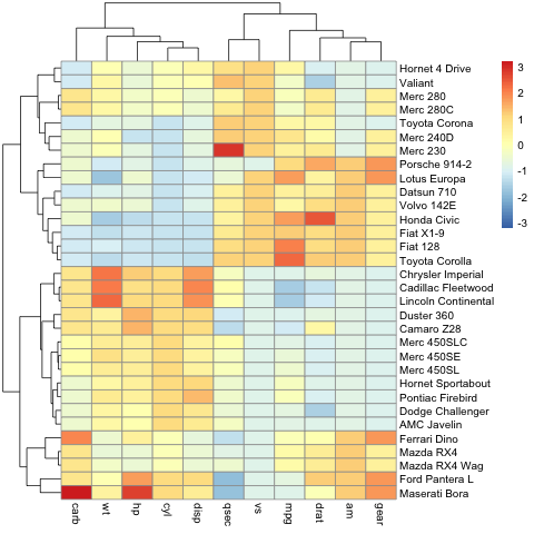
Heatmaps¶

Heatmaps are a grpahical means of displaying the results of agglomerative hierarchical clustering and a matrix of values (e.g. gene expression).

library(pheatmap)

pheatmap(mtcars, scale="column")