Hypothesis Testing and Power Calculations
One of things that R is used for is to perform simple testing and power calculations using canned functions. These functions are very simple to run; beign able to use and interpret them correctly is the hard part.
What is covered in this section
- Simple summary statistics
- Functions dealing with probability distributions
- Hypothesis testing
- Power / Sample size calculations
- Tabulating data
- Using simulations to calculate power (use of
forandif) - Customization of graphical plots
Set random see
set.seed(123)
Estimation
Often we want to estimate functions of data - for example, the mean or median of a set of numbers.
# First create a sample of 10 numbers from a normal distribution with mean 0 and sd 1
(x <- rnorm(10))
- 1.2369408226151
- 0.465511274432508
- 0.070684445387072
- 1.42149413805108
- -1.15858605831964
- 0.460407001136643
- -0.625685808667741
- 0.313346968415322
- -1.24274709077289
- -0.945266218602314
mean(x)
median(x)
sd(x)
var(x)
Hypothesis testing
Asssume theroy covered in morning statistics lecutres.
Example: Comparing group means
The t-test
x <- rnorm(mean=5.5, sd=1.5, n=10)
y <- rnorm(mean=5, sd=1.5, n=10)
result <- t.test(x, y, alternative = "two.sided", paired = FALSE,  var.equal = TRUE)
result
    Two Sample t-test

data:  x and y
t = 0.4472, df = 18, p-value = 0.6601
alternative hypothesis: true difference in means is not equal to 0
95 percent confidence interval:
 -1.105854  1.703865
sample estimates:
mean of x mean of y
 5.611938  5.312933
What is going on and what does all this actually mean?
The variable result is a list (similar to a hashmap or dictionary in
other languages), and named parts can be extracte with the $ method
- e.g. result$p.value gives the p-value.
The test firs cacluates a number called a \(t\) statistic that is given by some function of the data. From theoretical anaysis, we know that if the null hypothesis and assumptions of equal vairance and normal distributiono of the data are correct, then the \(t\) random variable will have a \(t\) distribution with 18 degrees of freedom (20 data points minus 2 estimated means).
The formula fot calcualting the \(t\)-statitic is
where \(\bar{x_1}\) and \(\bar{x_2}\) are the sample means, and se (standard error) is
where \(s_1^2\) and \(s_2^2\) are the sample variances.
We will calculate all these values to show what goes on in the sausage factory.
# These are custom R functions which we briefly showed you how to write in yesterday's session.

se <- function(x1, x2) {
    n1 <- length(x1)
    n2 <- length(x2)
    v1 <- var(x1)
    v2 <- var(x2)
    sqrt(v1/n1 + v2/n2)
    }
t <- function(x1, x2) {
    (mean(x1) - mean(x2))/se(x1, x2)
    }
t(x, y)
Now we will make use of our knowledge of probability distributions to understan what the p-value is.
We will plot the PDF of the t-distribution with df=18. The x-axis is the value of the t-statistic and the y-axis is the density (you can think of the density as the height of a histogram with total area normalized to sum to 1). The red lines are at the 2.5th and 97.5th quantiles - so for a two-sided test, the t-statistic must be more extreme than these two red lines (i.e. to the right of the 97.5th quantile or to the left of the 2.5th quantile) to reject the null hypothesis. We sse that our \(t\) statisitc (and its symmeetric negative) in dashed green do not meet this requirement - hence the p-value is > 0.05.
xp <- seq(-5, 5, length.out = 100)
plot(xp, dt(xp, df=18), type="l", col="blue")
score <- t(x, y)
abline(v=c(score, -score), col="green", lty=2)
thresholds <- c(qt(0.025, df=18), qt(0.975, df=18))
abline(v=thresholds, col="red", lty=1)
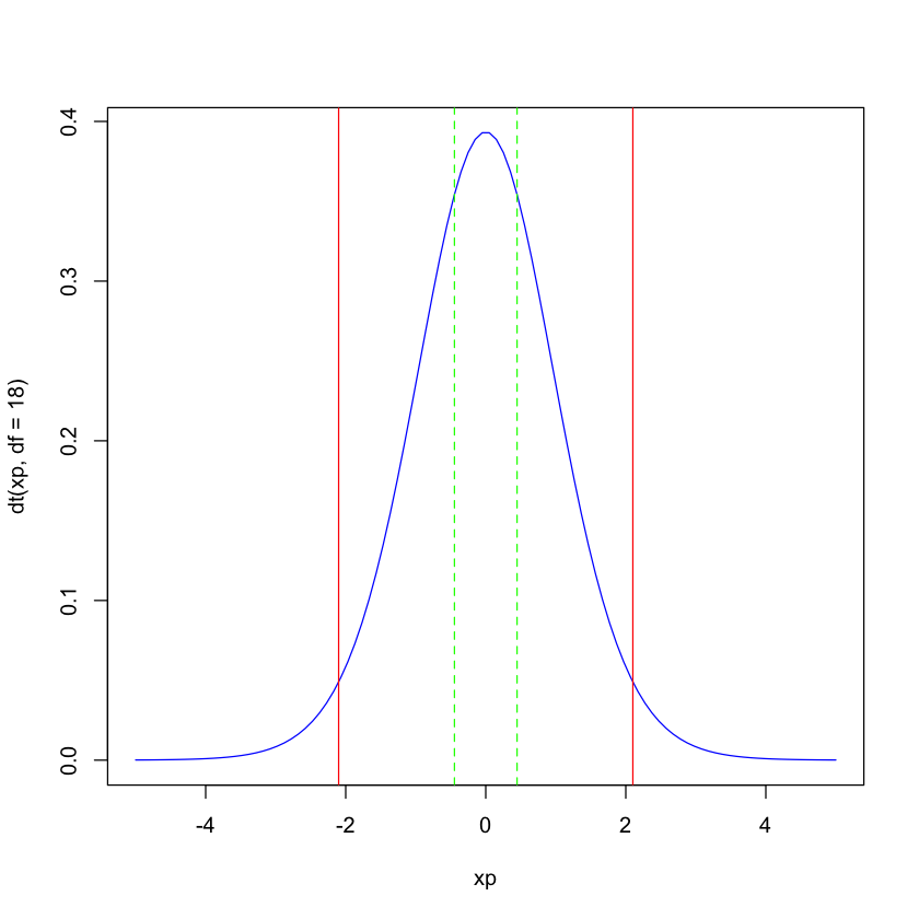
The p-value is the areau under the curve more extreme than the green lines. Since the t-statisic is positive, we can find the area to its right as one minus the cumulative density up to the value of the t-statitic. Doubling this (why?) gives us the p-value.
2*(1 - pt(score, df=18))
Note that this agrees with the value given by t.test.
The ranksum test
This calculates a test statistic \(W\) that is the sum of the outcomes for all pairwise comparisons of the ranks of the values in \(x\) and \(y\). Outcomes are 1 if the first item > the second item, 0.5 for a tie and 0 otherwise. This can be simplified to the follwoing formula
where \(R_1\) is the sum of ranks for the values in \(x\). For large samples, \(W\) can be considered to come from the normal distribution with means aand standard deviations that can be calculated from the data (look up by Googling or any mathematical statitics textbook if interested).
wilcox.test(x, y)
    Wilcoxon rank sum test

data:  x and y
W = 53, p-value = 0.8534
alternative hypothesis: true location shift is not equal to 0
Explicit calculation of statistic
w <- function(x, y) {
    r <- rank(c(x, y))
    nx <- length(x)
    sum(r[1:nx]) - nx*(nx+1)/2
    }
w(x, y)
Effect of sample size
x <- rnorm(mean=5.5, sd=1.5, n=200)
y <- rnorm(mean=5, sd=1.5, n=200)
t.test(x, y, )
    Welch Two Sample t-test

data:  x and y
t = 3.1236, df = 397.539, p-value = 0.001917
alternative hypothesis: true difference in means is not equal to 0
95 percent confidence interval:
 0.1676522 0.7370648
sample estimates:
mean of x mean of y
 5.474823  5.022465
wilcox.test(x, y)
    Wilcoxon rank sum test with continuity correction

data:  x and y
W = 23106, p-value = 0.007229
alternative hypothesis: true location shift is not equal to 0
Work!
Supppose we measure the weights of 100 people before and after a marathon. We want to know if there is a difference. What is the p-value for an appropirate parametric and non-parametric test?
before <- rnorm(n=100, mean=165, sd=25)
change <- rnorm(n=100, mean=-5, sd=10)
after <- before + change
# Parametric test
# Non-parametric test
Example: Comparing proportions
One sample
x <- sample(c('H', 'T'), 50, replace=TRUE)
table(x)
x
 H  T
26 24
binom.test(table(x), p = 0.5)
    Exact binomial test

data:  table(x)
number of successes = 26, number of trials = 50, p-value = 0.8877
alternative hypothesis: true probability of success is not equal to 0.5
95 percent confidence interval:
 0.3741519 0.6633949
sample estimates:
probability of success
                  0.52
Two samples
size = 50
x <- rbinom(n=1, prob=0.3, size=size)
y <- rbinom(n=1, prob=0.35, size=size)
(m <- matrix(c(x, y, size-x, size-y), ncol = 2))
| 10 | 40 |
| 16 | 34 |
prop.test(m)
    2-sample test for equality of proportions with continuity correction

data:  m
X-squared = 1.2994, df = 1, p-value = 0.2543
alternative hypothesis: two.sided
95 percent confidence interval:
 -0.31032527  0.07032527
sample estimates:
prop 1 prop 2
  0.20   0.32
Effect of sample size
size <- 500
x <- rbinom(n=1, prob=0.3, size=size)
y <- rbinom(n=1, prob=0.35, size=size)
(m <- matrix(c(x, y, size-x, size-y), ncol = 2))
| 155 | 345 |
| 193 | 307 |
Test that proportions are equal using z-score (prop.test)
prop.test(m)
    2-sample test for equality of proportions with continuity correction

data:  m
X-squared = 6.0336, df = 1, p-value = 0.01404
alternative hypothesis: two.sided
95 percent confidence interval:
 -0.13685795 -0.01514205
sample estimates:
prop 1 prop 2
 0.310  0.386
Alternative using \(\chi^2\) test
chisq.test(m)
    Pearson's Chi-squared test with Yates' continuity correction

data:  m
X-squared = 6.0336, df = 1, p-value = 0.01404
Work!
You find 3 circulating DNA fragments with the following properties
- fragment 1 has length 100 and is 35% CG
- fragment 2 has length 110 and is 40% CG
- fragment 3 has length 120 and is 50% GC
Do you reject the null hypotheses that the percent GC content is the same for all 3 fraemnets?
Sample size calculations
Need some explanation and disclaimers here!
See Qucik-R Power for more examples and more detailed explanation of function parameters.
install.packages("pwr", repos = "http://cran.r-project.org")
The downloaded binary packages are in
    /var/folders/xf/rzdg30ps11g93j3w0h589q780000gn/T//RtmpBJlIML/downloaded_packages
library(pwr)
Warning message:
: package ‘pwr’ was built under R version 3.1.3
For simple power calculations, you need 3 out of 4 of the follwoing: - n = number of samples / experimental units - sig.level = what “p-value” you will be using to determine significance - power = fraction of experiments that will reject null hypothesis - d = “effect size” ~ depends on context
d <- (5.5 - 5.0)/1.5
pwr.t.test(d = d, sig.level = 0.05, power = 0.8)
     Two-sample t test power calculation

              n = 142.2462
              d = 0.3333333
      sig.level = 0.05
          power = 0.8
    alternative = two.sided

NOTE: n is number in each group
p1 = 0.30
p2 = 0.35
(h = abs(2*asin(p1) - 2*asin(p2)))

pwr.2p.test(h = h, sig.level = 0.05, power = 0.9)
     Difference of proportion power calculation for binomial distribution (arcsine transformation)

              h = 0.1057569
              n = 1878.922
      sig.level = 0.05
          power = 0.9
    alternative = two.sided

NOTE: same sample sizes
Check our understanding of what power means
Note: The code below is an example of a statistical simulation. It can be made more efficient by vectorization, but looping is initially easer to understand and the speed makes no practical differnece for such a small exmaple.
Before running the code - try to answer this question:
If we performed the same experiment 1000 times with n=1879 (from power calucations above), how many experiments would yield a p-value of less than 0.05?
size <- 1879
hits <- 0
ntrials <- 1000
for (i in 1:ntrials) {
    x <- rbinom(n=1, prob=0.3, size=size)
    y <- rbinom(n=1, prob=0.35, size=size)
    m <- matrix(c(x, y, size-x, size-y), ncol = 2)
    result <- prop.test(m)
    hits <- hits + (result$p.value < 0.05)
    }
hits/ntrials
Work!
Suppose an investigator proposes to use an unpaired t-test to examine differences between two groups of size 13 and 16. What is the power at the usual 0.05 significance level for effet sizes of 0.1, 0.5 and 1.0.