Introduction to DESeq2
This notebook serves as a tutorial for using the DESeq2 package. Please be sure to consult the excellent vignette provided by the DESeq2 package. Hopefully, we will also get a chance to review the edgeR package (which also has a very nice vignette which I suggest that you review)
Load packages
Load requisite R packages
library(DESeq2)
library(tools)
options(width=100)
Error in library(DESeq2): there is no package called ‘DESeq2’
Importing and Inspecting Data
Let’s set the file name containing the phenotype data and the directory storing the count files from the htseq-count step. You will have to adjust these strings. Note that it is assumed that all count files are stored under a single directory.
phfile="sampletable.txt"
cntdir="/home/owzar001/CURRENT/summercourse-2015/Data/COUNTS"
Next, read in the phenotype data from the sample file. It is always a good idea to display the md5sum hash key for the file. Note that when importing the file using read.table(), the stringsAsFactor argument is set to FALSE. This imports strings as character rather than factor objects.
md5sum(phfile)
phdata=read.table(phfile,sep=",",stringsAsFactor=FALSE)
It is always a good idea to check the dimension of the file you have read in
dim(phdata)
- 6
- 3
Finally, it is a good idea to print out the sample data (or at least the first few rows)
phdata
| V1 | V2 | V3 | |
|---|---|---|---|
| 1 | AGTCAA_counts.tsv | AGTCAA | 0 |
| 2 | AGTTCC_counts.tsv | AGTTCC | 0 |
| 3 | ATGTCA_counts.tsv | ATGTCA | 0 |
| 4 | CCGTCC_counts.tsv | CCGTCC | 1 |
| 5 | GTCCGC_counts.tsv | GTCCGC | 1 |
| 6 | GTGAAA_counts.tsv | GTGAAA | 1 |
Next, we reformat the phenotype data object with more informative column names and by adding the md5sum hash keys for the count files. When dealing with directory and file names you should use file.path(), dirname() and basename(). Check out the help files
colnames(phdata)=c("filename","sampid","trt")
phdata[["md5sum"]]=md5sum(file.path(cntdir,phdata[["filename"]]))
phdata
| filename | sampid | trt | md5sum | |
|---|---|---|---|---|
| 1 | AGTCAA_counts.tsv | AGTCAA | 0 | NA |
| 2 | AGTTCC_counts.tsv | AGTTCC | 0 | NA |
| 3 | ATGTCA_counts.tsv | ATGTCA | 0 | NA |
| 4 | CCGTCC_counts.tsv | CCGTCC | 1 | NA |
| 5 | GTCCGC_counts.tsv | GTCCGC | 1 | NA |
| 6 | GTGAAA_counts.tsv | GTGAAA | 1 | NA |
The first step to an analysis using the DESeq2 package is to import the raw counts. If these counts stored in files generated by htseq-count, then you may use the DESeqDataSetFromHTSeqCount() function from the package. This function expects a sample table that contains the sample id in the first column and the count file name in teh second column. Our sample table is not in that format. It is easy to reorder the columns
phdata=phdata[c("sampid","filename","trt","md5sum")]
phdata
| sampid | filename | trt | md5sum | |
|---|---|---|---|---|
| 1 | AGTCAA | AGTCAA_counts.tsv | 0 | NA |
| 2 | AGTTCC | AGTTCC_counts.tsv | 0 | NA |
| 3 | ATGTCA | ATGTCA_counts.tsv | 0 | NA |
| 4 | CCGTCC | CCGTCC_counts.tsv | 1 | NA |
| 5 | GTCCGC | GTCCGC_counts.tsv | 1 | NA |
| 6 | GTGAAA | GTGAAA_counts.tsv | 1 | NA |
Also, DESeq2 prefers that the treatment variable is of factor class. So we will convert it
phdata[["trt"]]=as.factor(phdata[["trt"]])
Now, we import the counts. Note that the first argument is the sample table while the second is the directory storing the count files. The last argument specifies the design. More on this later.
dds=DESeqDataSetFromHTSeqCount(sampleTable = phdata,directory = cntdir,design=~trt)
Error in eval(expr, envir, enclos): could not find function "DESeqDataSetFromHTSeqCount"
Inspect object
Let’s has a look at the object we have created.
dds
Error in eval(expr, envir, enclos): object 'dds' not found
Note that this object is of class DESeqDataSet. It contains data on 4436 genes on 6 samples. Use the colData() function to see what you have read in
colData(dds)
Error in eval(expr, envir, enclos): could not find function "colData"
The first thing you may want to do is to have a look at the raw counts you have imported. You can use the counts(). Let’s looks the first three genes (use the head() function to avoid printing out all genes). Before that notw the dimension of the count matrix (does it look correct?)
dim(counts(dds))
Error in eval(expr, envir, enclos): could not find function "counts"
Now print the raw counts for the first three genes (how can you verify this looking at the files from htseq-count)
head(counts(dds),3)
Error in head(counts(dds), 3): could not find function "counts"
8Slots of an S4 class
To get the slots of an S4 class use slotNames()
slotNames(dds)
Error in is(x, "classRepresentation"): object 'dds' not found
Now let’s look at a few slots:
This gives the design of the study
Error in parse(text = x, srcfile = src): <text>:1:6: unexpected symbol
1: This gives
         ^
dds@design
Error in eval(expr, envir, enclos): object 'dds' not found
The dispersion function is NULl for now (more on this later)
dds@dispersionFunction
Error in eval(expr, envir, enclos): object 'dds' not found
This slots return gene specific information (it will be populated later)
dds@rowData
Error in eval(expr, envir, enclos): object 'dds' not found
This slot returns the sample data
dds@colData
Error in eval(expr, envir, enclos): object 'dds' not found
Before, going to the next step, let’s look at the output from mcols()
mcols(dds)
Error in eval(expr, envir, enclos): could not find function "mcols"
Estimate Size Factors and Dispersion Parameters
You recall that DESeq requires that we have estimates for sample specific size factors and gene specific dispersion factors. More specifically, recall that DESeq models the count \(K_{ij}\) (gene \(i\), sample \(j\)) as negative binomial with mean \(\mu_{ij}\) and dispersion parameter \(\alpha_i\). Here \(\mu_{ij}=s_j q_{ij}\) where \(\log_2(q_{ij}) = \beta_{0i} + \beta_{1i} z_j\). Here \(s_j\) is the sample \(j\) specific size factor.
Size Factors
We begin by estimating the size factors \(s_1,\ldots,s_6\):
dds <- estimateSizeFactors(dds)
Error in eval(expr, envir, enclos): could not find function "estimateSizeFactors"
Now, compare the dds object to that of before applying the estimateSizeFactors() function. What has changed? What remains unchanged?
dds
Error in eval(expr, envir, enclos): object 'dds' not found
Note that there is a sizeFactor added to colData. Let’s look at it more carefully
colData(dds)
Error in eval(expr, envir, enclos): could not find function "colData"
You can also get the size factors directly (why are there six size factors?)
sizeFactors(dds)
Error in eval(expr, envir, enclos): could not find function "sizeFactors"
It is preferable to limit the number of decimal places. Next show the size factors rounded to 3 decimal places
round(sizeFactors(dds),3)
Error in eval(expr, envir, enclos): could not find function "sizeFactors"
Now that the size factors have been estimated, we can get “normalized” counts
head(counts(dds),3)
head(counts(dds,normalize=TRUE),3)
Error in head(counts(dds), 3): could not find function "counts"
Error in head(counts(dds, normalize = TRUE), 3): could not find function "counts"
Note that these are the counts divided by the size factors. Compare the first row of the last table (“normalized” counts for gene 1) to the hand calculation below.
counts(dds)[1,]/sizeFactors(dds)
Error in eval(expr, envir, enclos): could not find function "counts"
Exercise: How do you get the raw counts for gene “GeneID:12930116”?
counts(dds)["GeneID:12930116",]
Error in eval(expr, envir, enclos): could not find function "counts"
Exercise: How do you get the normalized counts for gene “GeneID:12930116”?
counts(dds,normalize=TRUE)["GeneID:12930116",]
Error in eval(expr, envir, enclos): could not find function "counts"
Exercise: Get a summary (mean, median, quantiles etc ) of the size factors
summary(sizeFactors(dds))
Error in summary(sizeFactors(dds)): could not find function "sizeFactors"
Before going to the next step, let’s look at the dispersionFunction slot
dds@dispersionFunction
Error in eval(expr, envir, enclos): object 'dds' not found
Dispersion Parameters
Next, we get the dispersion factors \(\alpha_1,\ldots,\alpha_{4436}\)
dds=estimateDispersions(dds)
Error in eval(expr, envir, enclos): could not find function "estimateDispersions"
Now inspect the dds object again and note that the rowRanges slot has extra information (“metadata column names(0):” before versus “column names(9): baseMean baseVar ... dispOutlier dispMAP”)
dds
Error in eval(expr, envir, enclos): object 'dds' not found
We can extract the gene specific dispersion factors using dispersions(). Note that there will be one number per gene. We look at the first four genes (rounded to 4 decimal places)
alphas=dispersions(dds)
Error in eval(expr, envir, enclos): could not find function "dispersions"
Verify that the number of dispersion factors equals the number of genes
length(alphas)
Error in eval(expr, envir, enclos): object 'alphas' not found
Print the dispersion factors for the first 5 genes rounded to four decimal points
round(alphas[1:5],4)
Error in eval(expr, envir, enclos): object 'alphas' not found
Extract the metadata using mcols() for the first four genes (recall that it was previously
mcols(dds)[1:4,]
Error in eval(expr, envir, enclos): could not find function "mcols"
Exercise: Provide statistical summaries of the dispersion factors
summary(dispersions(dds))
Error in summary(dispersions(dds)): could not find function "dispersions"
Exercise: Summarize the dispersion factors using a box plot (may want to log transform)
boxplot(log(dispersions(dds)))

Error in boxplot(log(dispersions(dds))): could not find function "dispersions"
Differential Expression Analysis
We can now conduct a differential expression analysis using the DESeq() function. Keep in mind that to get to this step, we first estimated the size factors and then the dispersion parameters.
ddsDE=DESeq(dds)
Error in eval(expr, envir, enclos): could not find function "DESeq"
We can get the results for the differential expression analysis using results()
myres=results(ddsDE)
Error in eval(expr, envir, enclos): could not find function "results"
Let’s look at the results for the first four genes
myres[1:4,]
Error in eval(expr, envir, enclos): object 'myres' not found
Calculate BH adjusted P-values by “hand” using the p.adjust() function
BH=p.adjust(myres$pvalue,"BH")
BH[1:4]
Error in p.adjust(myres$pvalue, "BH"): object 'myres' not found
Error in eval(expr, envir, enclos): object 'BH' not found
You can get the descriptions for the columns from the DE analysis
data.frame(desc=mcols(myres)$description)
Error in data.frame(desc = mcols(myres)$description): could not find function "mcols"
We can get summaries of the results:
summary(myres,0.05)
Error in summary(myres, 0.05): object 'myres' not found
You can sort the results by say the unadjusted P-values
myres[order(myres[["pvalue"]])[1:4],]
Error in eval(expr, envir, enclos): object 'myres' not found
To get the list of genes with unadjusted P-values < 0.00001 and absolute log2 FC of more than 4
subset(myres,pvalue<0.00001&abs(log2FoldChange)>4)
Error in subset(myres, pvalue < 1e-05 & abs(log2FoldChange) > 4): object 'myres' not found
To get the list of genes with unadjusted P-values < 0.00001 and upregulated genes with log2 FC of more than 4
subset(myres,pvalue<0.00001&log2FoldChange>4)
Error in subset(myres, pvalue < 1e-05 & log2FoldChange > 4): object 'myres' not found
The P-values for the four top genes are beyond machine precision. You can use the format.pval() function to properly format the P-values. PLEASE promote ending the practice of publishing P-values below machine precision. (that would be akin to stating the weight of an object that weighs less than one pound with scale that whose minimum weight spec is 1lbs).
myres$pval=format.pval(myres$pvalue)
myres[order(myres[["pvalue"]])[1:4],]
Error in format.pval(myres$pvalue): object 'myres' not found
Error in eval(expr, envir, enclos): object 'myres' not found
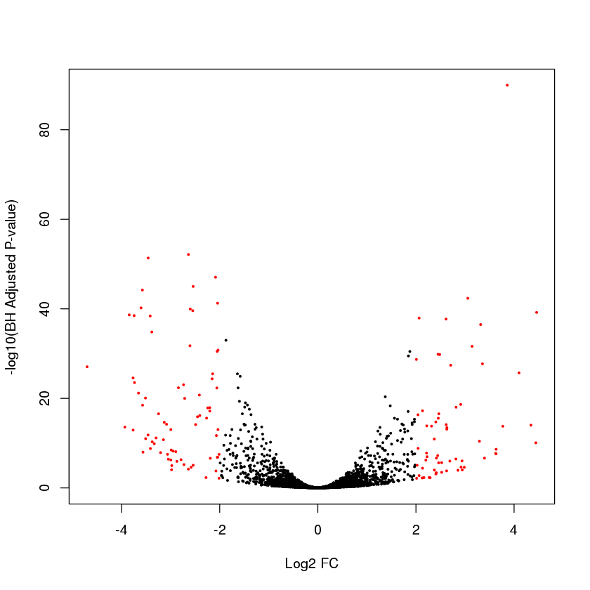
Let’s look at a volcano plot
plot(myres$log2FoldChange,-log10(myres$padj),pch=19,cex=0.3,xlab="Log2 FC",ylab="-log10(BH Adjusted P-value)")

Error in plot(myres$log2FoldChange, -log10(myres$padj), pch = 19, cex = 0.3, : object 'myres' not found
Extract results for genes GeneID:12932226 and GeneID:12930116
myres[c("GeneID:12932226","GeneID:12930116"),]
Error in eval(expr, envir, enclos): object 'myres' not found
Exercise: Annotate the hits with adjusted P-values < 0.05 and absolute log2 FC greater than 2 in red
plot(myres$log2FoldChange,-log10(myres$padj),pch=19,cex=0.3,xlab="Log2 FC",ylab="-log10(BH Adjusted P-value)",col=ifelse(myres$padj<0.05&abs(myres$log2FoldChange)>2,"red","black"))
Error in plot(myres$log2FoldChange, -log10(myres$padj), pch = 19, cex = 0.3, : object 'myres' not found
Converting/Normalizing Counts to “Expressions”
Normalized Counts
We have already shown how to “normalize” the counts using the estimated size factors
head(counts(dds,normalize=TRUE),3)
Error in head(counts(dds, normalize = TRUE), 3): could not find function "counts"
Plot the counts stratified by treatment for the 2nd gene
plotCounts(dds, 2,intgroup="trt")

Error in eval(expr, envir, enclos): could not find function "plotCounts"
Or alternatively (better)
plotCounts(dds, "GeneID:12930115",intgroup="trt")

Error in eval(expr, envir, enclos): could not find function "plotCounts"
Now get this plot for the top hit
plotCounts(dds, "GeneID:12931678",intgroup="trt")

Error in eval(expr, envir, enclos): could not find function "plotCounts"
FPM
Another approach is to FPM: fragments per million mapped fragments
Error in parse(text = x, srcfile = src): <text>:1:9: unexpected symbol
1: Another approach
            ^
head(fpm(dds),3)
Error in head(fpm(dds), 3): could not find function "fpm"
Let’s calculate the FPM manually. For gene \(i\) sample \(j\), the FPM is defined as \(\frac{K_{ij}}{D_j}\times 10^{6}\) where \(D_j=\sum_{i=1} K_{ij}\) is the read depth for sample \(j\). First get the read depth for each sample
D=colSums(counts(dds))
D
Error in is.data.frame(x): could not find function "counts"
function (expr, name)
.External(C_doD, expr, name)
By default, the fpm() function uses a robust approach. We will disable this right now as to replicate the standard FPM. Let’s look at gene 1
fpm1=fpm(dds,robust=FALSE)[1,]
fpm1
Error in eval(expr, envir, enclos): could not find function "fpm"
Error in eval(expr, envir, enclos): object 'fpm1' not found
Now get the raw counts for gene 1
cnt1=counts(dds)[1,]
cnt1
Error in eval(expr, envir, enclos): could not find function "counts"
Error in eval(expr, envir, enclos): object 'cnt1' not found
Now calculate the FPM for gene 1
myfpm1=cnt1/D*1e6
myfpm1
Error in eval(expr, envir, enclos): object 'cnt1' not found
Error in eval(expr, envir, enclos): object 'myfpm1' not found
This is how you check if two numeric columns are “equal”
min(abs(fpm1-myfpm1))
Error in eval(expr, envir, enclos): object 'fpm1' not found
FPKM
To calculate the FPKM (fragments per kilobase per million mapped fragments) we need to add annotation to assign the feature lengths. More specifically, for gene \(i\) sample \(j\), the FPKM is defined as \(\frac{K_{ij}}{\ell_i D_j}\times 10^3 \times 10^{6}\) where \(\ell_i\) is the “length” of gene \(i\) (fragments for each \(10^3\) bases in the gene for every \(\frac{D_j}{10^6}\) fragments. More on this later.
Regularized log transformation
The regularized log transform can be obtained using the rlog() function. Note that an important argument for this function is blind (TRUE by default). The default “blinds” the normalization to the design. This is very important so as to not bias the analyses (e.g. class discovery
rld=rlog(dds,blind=TRUE)
Error in eval(expr, envir, enclos): could not find function "rlog"
Hierarchical clustering using rlog transformation
dists=dist(t(assay(rld)))
plot(hclust(dists))

Error in t(assay(rld)): could not find function "assay"
Error in hclust(dists): object 'dists' not found
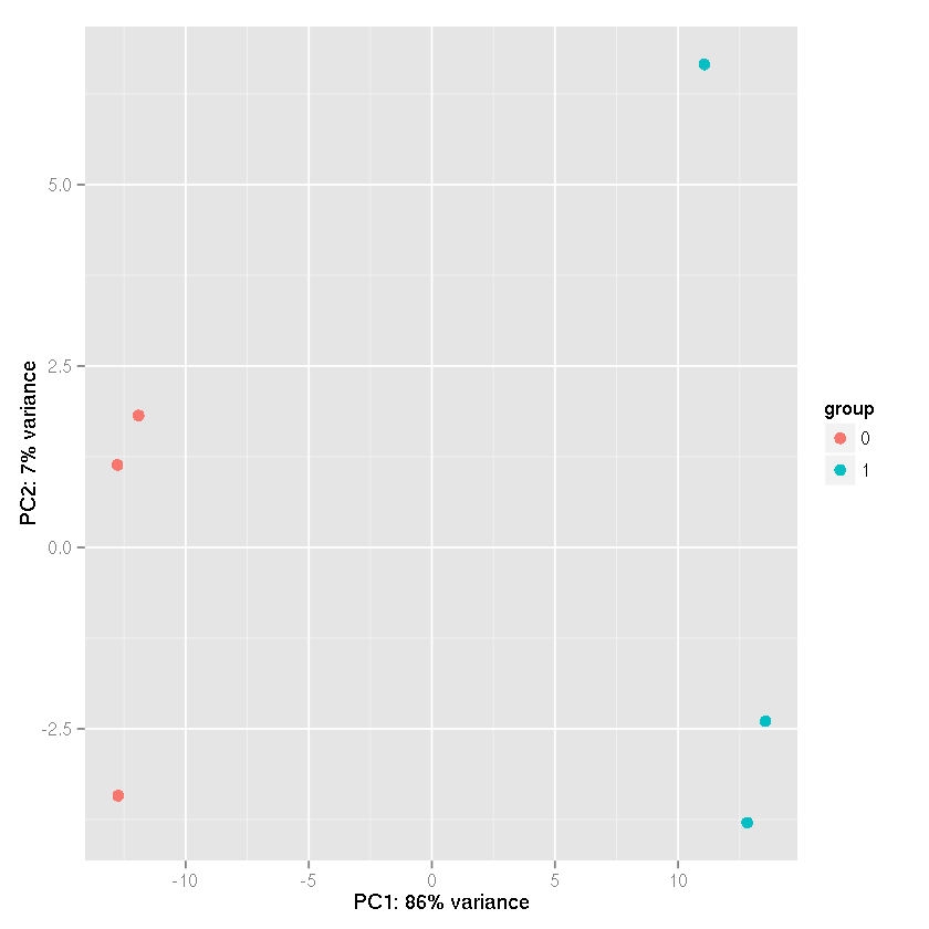
PC Analysis using the rlog transformation
plotPCA(rld,intgroup="trt")
Error in eval(expr, envir, enclos): could not find function "plotPCA"
sessionInfo()
R version 3.1.2 (2014-10-31)
Platform: x86_64-apple-darwin13.4.0 (64-bit)

locale:
[1] en_US.UTF-8/en_US.UTF-8/en_US.UTF-8/C/en_US.UTF-8/en_US.UTF-8

attached base packages:
[1] tools     stats     graphics  grDevices utils     datasets  methods   base

loaded via a namespace (and not attached):
 [1] base64enc_0.1-3      digest_0.6.8         evaluate_0.7.2       IRdisplay_0.3.0.9000
 [5] IRkernel_0.3.0.9000  jsonlite_0.9.17      magrittr_1.5         repr_0.1.0.9000
 [9] rzmq_0.7.7           stringi_0.5-5        stringr_1.0.0        uuid_0.1-2
Import count data using basic tools
We want to read in the count files using more basic tools (important if the count files are not generated fro,m htseq-count). We will import the files as matrices. We start with some of the preliminary steps
library(tools)
phfile="/home/owzar001/CURRENT/summercourse-2015/Data/sampletable.txt"
cntdir="/home/owzar001/CURRENT/summercourse-2015/Data/COUNTS"
md5sum(phfile)
phdata=read.table(phfile,sep=",",stringsAsFactor=FALSE)
colnames(phdata)=c("filename","sampid","trt")
phdata[["md5sum"]]=md5sum(file.path(cntdir,phdata[["filename"]]))
phdata
| filename | sampid | trt | md5sum | |
|---|---|---|---|---|
| 1 | AGTCAA_counts.tsv | AGTCAA | 0 | a9eaa959aba1b02b3831583c2a9751c8 |
| 2 | AGTTCC_counts.tsv | AGTTCC | 0 | 4183767e4eeb75dc582bcf438af13500 |
| 3 | ATGTCA_counts.tsv | ATGTCA | 0 | 26fbba06520758e5a3acd9bd432ebed4 |
| 4 | CCGTCC_counts.tsv | CCGTCC | 1 | 50036a88fd48645f740a31f4f4352cfb |
| 5 | GTCCGC_counts.tsv | GTCCGC | 1 | bb1cecd886127159157e9431d072cad5 |
| 6 | GTGAAA_counts.tsv | GTGAAA | 1 | fa544c0a076eedb54937c7189f4e1fbc |
phdata=phdata[c("sampid","filename","trt","md5sum")]
phdata
| sampid | filename | trt | md5sum | |
|---|---|---|---|---|
| 1 | AGTCAA | AGTCAA_counts.tsv | 0 | a9eaa959aba1b02b3831583c2a9751c8 |
| 2 | AGTTCC | AGTTCC_counts.tsv | 0 | 4183767e4eeb75dc582bcf438af13500 |
| 3 | ATGTCA | ATGTCA_counts.tsv | 0 | 26fbba06520758e5a3acd9bd432ebed4 |
| 4 | CCGTCC | CCGTCC_counts.tsv | 1 | 50036a88fd48645f740a31f4f4352cfb |
| 5 | GTCCGC | GTCCGC_counts.tsv | 1 | bb1cecd886127159157e9431d072cad5 |
| 6 | GTGAAA | GTGAAA_counts.tsv | 1 | fa544c0a076eedb54937c7189f4e1fbc |
phdata[["trt"]]=as.factor(phdata[["trt"]])
This function reads the data from one file and returns the results as a matrix. It is designed to only keep the rows for which the gene id starts with the prefix “GeneID”
readcnts=function(fname,sep="\t",prefix="GeneID",collab="V1",header=FALSE)
    {
        ### Import text file
        dat=read.table(fname,sep=sep,header=header,stringsAsFactor=FALSE)
        ### Only keep rows for which the gene id matches with the prefix
        dat=dat[substr(dat[[collab]],1,nchar(prefix))==prefix,]
        return(dat)
    }
Let’s read in a file
file1=readcnts("/home/owzar001/CURRENT/summercourse-2015/Data/COUNTS/AGTCAA_counts.tsv")
dim(file1)
- 4436
- 2
head(file1)
| V1 | V2 | |
|---|---|---|
| 1 | GeneID:12930114 | 118 |
| 2 | GeneID:12930115 | 30 |
| 3 | GeneID:12930116 | 15 |
| 4 | GeneID:12930117 | 12 |
| 5 | GeneID:12930118 | 122 |
| 6 | GeneID:12930119 | 60 |
Now read in all files
## Read in the first file
countdat=readcnts(file.path(cntdir,phdata$filename[1]))
### Assign the sample id as the column name
names(countdat)[2]=phdata$sampid[1]
### Repeat the last two steps for files 2 ... 6 and merge
### along each step
for(i in 2:nrow(phdata))
    {
        dat2=readcnts(file.path(cntdir,phdata$filename[i]))
        names(dat2)[2]=phdata$sampid[i]
        countdat=merge(countdat,dat2,by="V1")
    }

geneid=countdat$V1
countdat=as.matrix(countdat[,-1])
row.names(countdat)=geneid
head(countdat)
| AGTCAA | AGTTCC | ATGTCA | CCGTCC | GTCCGC | GTGAAA | |
|---|---|---|---|---|---|---|
| GeneID:12930114 | 118 | 137 | 149 | 120 | 161 | 174 |
| GeneID:12930115 | 30 | 42 | 25 | 18 | 32 | 34 |
| GeneID:12930116 | 15 | 55 | 37 | 49 | 36 | 27 |
| GeneID:12930117 | 12 | 12 | 13 | 11 | 7 | 6 |
| GeneID:12930118 | 122 | 137 | 94 | 48 | 131 | 69 |
| GeneID:12930119 | 60 | 88 | 78 | 53 | 43 | 29 |
library(DESeq2)
Loading required package: S4Vectors
Loading required package: stats4
Loading required package: BiocGenerics
Loading required package: parallel

Attaching package: ‘BiocGenerics’

The following objects are masked from ‘package:parallel’:

    clusterApply, clusterApplyLB, clusterCall, clusterEvalQ,
    clusterExport, clusterMap, parApply, parCapply, parLapply,
    parLapplyLB, parRapply, parSapply, parSapplyLB

The following object is masked from ‘package:stats’:

    xtabs

The following objects are masked from ‘package:base’:

    anyDuplicated, append, as.data.frame, as.vector, cbind, colnames,
    do.call, duplicated, eval, evalq, Filter, Find, get, intersect,
    is.unsorted, lapply, Map, mapply, match, mget, order, paste, pmax,
    pmax.int, pmin, pmin.int, Position, rank, rbind, Reduce, rep.int,
    rownames, sapply, setdiff, sort, table, tapply, union, unique,
    unlist, unsplit

Creating a generic function for ‘nchar’ from package ‘base’ in package ‘S4Vectors’
Loading required package: IRanges
Loading required package: GenomicRanges
Loading required package: GenomeInfoDb
Loading required package: Rcpp
Loading required package: RcppArmadillo
dds=DESeqDataSetFromMatrix(countdat,DataFrame(phdata),design=~trt)
dds
class: DESeqDataSet
dim: 4436 6
exptData(0):
assays(1): counts
rownames(4436): GeneID:12930114 GeneID:12930115 ... GeneID:13406005
  GeneID:13406006
rowRanges metadata column names(0):
colnames(6): AGTCAA AGTTCC ... GTCCGC GTGAAA
colData names(4): sampid filename trt md5sum
sessionInfo()
R version 3.2.1 (2015-06-18)
Platform: x86_64-pc-linux-gnu (64-bit)
Running under: Debian GNU/Linux 8 (jessie)

locale:
 [1] LC_CTYPE=en_US.UTF-8       LC_NUMERIC=C
 [3] LC_TIME=en_US.UTF-8        LC_COLLATE=en_US.UTF-8
 [5] LC_MONETARY=en_US.UTF-8    LC_MESSAGES=en_US.UTF-8
 [7] LC_PAPER=en_US.UTF-8       LC_NAME=C
 [9] LC_ADDRESS=C               LC_TELEPHONE=C
[11] LC_MEASUREMENT=en_US.UTF-8 LC_IDENTIFICATION=C

attached base packages:
 [1] parallel  stats4    tools     stats     graphics  grDevices utils
 [8] datasets  methods   base

other attached packages:
[1] DESeq2_1.8.1              RcppArmadillo_0.5.200.1.0
[3] Rcpp_0.11.6               GenomicRanges_1.20.5
[5] GenomeInfoDb_1.4.1        IRanges_2.2.5
[7] S4Vectors_0.6.2           BiocGenerics_0.14.0

loaded via a namespace (and not attached):
 [1] RColorBrewer_1.1-2   futile.logger_1.4.1  plyr_1.8.3
 [4] XVector_0.8.0        futile.options_1.0.0 base64enc_0.1-3
 [7] rpart_4.1-9          digest_0.6.8         uuid_0.1-2
[10] RSQLite_1.0.0        annotate_1.46.1      lattice_0.20-31
[13] jsonlite_0.9.16      evaluate_0.7         gtable_0.1.2
[16] DBI_0.3.1            IRdisplay_0.3        IRkernel_0.4
[19] proto_0.3-10         gridExtra_2.0.0      rzmq_0.7.7
[22] genefilter_1.50.0    cluster_2.0.1        repr_0.3
[25] stringr_1.0.0        locfit_1.5-9.1       nnet_7.3-9
[28] grid_3.2.1           Biobase_2.28.0       AnnotationDbi_1.30.1
[31] XML_3.98-1.3         survival_2.38-2      BiocParallel_1.2.9
[34] foreign_0.8-63       latticeExtra_0.6-26  Formula_1.2-1
[37] geneplotter_1.46.0   ggplot2_1.0.1        reshape2_1.4.1
[40] lambda.r_1.1.7       magrittr_1.5         splines_3.2.1
[43] scales_0.2.5         Hmisc_3.16-0         MASS_7.3-40
[46] xtable_1.7-4         colorspace_1.2-6     stringi_0.5-5
[49] acepack_1.3-3.3      munsell_0.4.2