Using R for supervised learning
This notebook goes over the basic concept of how to construct and use a supervised learning pipleine for classificaioon. We will use the k-nearest neighbors algorithm for illustration, but the baisc ideas carry over to all algorithms for classificaiton and regression.
healthdy <- read.table('healthdy.txt', header = TRUE)
head(healthdy)
| ID | GENDER | FLEXPRE | FLEXPOS | BAWPRE | BAWPOS | BWWPRE | BWWPOS | BFPPRE | BFPPOS | FVCPRE | FVPOS | METSPRE | METSPOS | |
|---|---|---|---|---|---|---|---|---|---|---|---|---|---|---|
| 1 | 0 | 1 | 21.000 | 21.500 | 70.5 | 75.6 | 3.3 | 3.7 | 14.58 | 14.17 | 5.1 | 5.1 | 12.7 | 18.0 |
| 2 | 2 | 1 | 21.000 | 21.250 | 71.3 | 70.7 | 3.2 | 3.6 | 16.79 | 13.95 | 4.3 | 4.3 | 11.1 | 12.0 |
| 3 | 3 | 1 | 21.500 | 20.000 | 64.5 | 66.6 | 4.1 | 4.0 | 6.6 | 08.98 | 4.5 | 4.5 | 15.3 | 16.7 |
| 4 | 4 | 1 | 23.000 | 23.375 | 97 | 95.0 | 4.4 | 4.3 | 18.04 | 17.32 | 4.7 | 4.3 | 12.0 | 17.5 |
| 5 | 5 | 1 | 21.000 | 21.000 | 71 | 73.2 | 3.7 | 3.8 | 11.12 | 11.50 | 5.8 | 5.8 | 12.2 | 12.2 |
| 6 | 6 | 1 | 20.500 | 20.750 | 72.5 | 73.1 | 3.1 | 3.4 | 17.88 | 16.22 | 4.3 | 4.3 | 11.1 | 10.0 |
Data from Health Dynamics class at Hope College–collected about 1985 by Gregg Afman. Downloaded from http://www.math.hope.edu/swanson/data/healthdy.txt
Gender 1 = Male Gender 2 = Female
Flexpre = Flexability at the beginning of the semester Flexpro = Flexability at the end of the semester
Bawpre = Air Weight at the beginning of the semester Bawpro = Air weight at the end of the semester
Bwwpre = Water weight at the beginning of the semester Bwwpro = Water weight at the end of the semester
Bfppre = Body fat at the beginning of the semester Bfppro = Body fat at the end of the semester
Fvcpre = Forced capacity at the beginning of the semester Fvcpro = Forced capacity at the end of the semester
Metspre = Mets at the beginning of the semester Metspro = Mets at the end of the semester
Supervised learning problem
For simplicity and ease of visualization, we will just use the first 2 indepdendent variables as fearures for predicitng gender. In practice, the selection of approprieate features to use as predictors can be a challenging problem that greatly affects the effectiveness of supervised learning.
So the problme is: How accurately can we guess the gender of a student from the Flexpre and Bawpre variables?
Visualizing the data
First let’s make a smaller dataframe containing just the variables of interest, and make some plots.
df <- healthdy[,c("ID", "GENDER", "FLEXPRE", "BAWPRE")]
df$ID <- factor(df$ID)
df$GENDER <- factor(df$GENDER, labels = c("Male", "Female"))
df$FLEXPRE <- as.numeric(df$FLEXPRE)
summary(df)
      ID         GENDER       FLEXPRE          BAWPRE
0      :  2   Male  : 82   Min.   : 1.00   Min.   :35.20
2      :  2   Female:100   1st Qu.:26.00   1st Qu.:57.73
3      :  2                Median :42.00   Median :65.05
4      :  2                Mean   :38.76   Mean   :66.99
5      :  2                3rd Qu.:52.00   3rd Qu.:74.50
6      :  2                Max.   :67.00   Max.   :98.50
(Other):170
Let’s check the mean flexibilitiy and weights for boys and girls.
with(df, aggregate(df[,3:4], by=list(Gender=GENDER), FUN=mean))
| Gender | FLEXPRE | BAWPRE | |
|---|---|---|---|
| 1 | Male | 33.46341 | 75.89024 |
| 2 | Female | 43.1 | 59.695 |
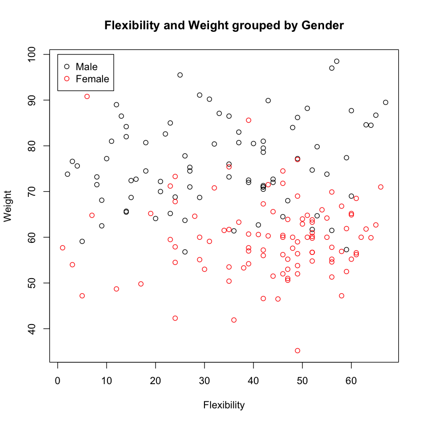
On average, girls are more flexible and weigh less than boys. This is confirmed viually.
plot(df$FLEXPRE, df$BAWPRE, col=df$GENDER,
     xlab="Flexibility", ylab="Weight",
     main="Flexibility and Weight grouped by Gender")
legend(0, 100, c("Male", "Female"), pch=1, col=1:2)
Comments
It looks like there is a pretty good probablility that we can guess the gender from the body weight and flexibilty alone. The k-nearest neighbor does this guessing in a very simple fashion - Given any point in the data set, it looks for the nearest k neighboring points, and simply uses the majority gender among these neighbors as the guess. In the sections below, we’ll implement a supervised learnign pipeline using k-nearest neighbors.
Work!
Review questions to make sure you are up to speed with basic data manipulation and plotting.
Q1. Tabulate the median value of FLEXPRE and BAWPRE by gender.
Q2. Tabluate the average change in weight from the beginnig to the end of the semester by gender.
Q3. Identify from the plot above the IDs of 3 individuals for whom you expect k-nearest neighbors to make the wrong gender prediction. HInt: Make a scatterplot but add the IDs as labels for each point, using a small x-offset of 2.5 so that labels are immediately to the right of each point.
Splitting data into training and test data sets
We will use 3/4 of the data to train the algorithm and 1/4 to test how good it is. The reason for doing this is that if we train on the full data set, the algorithm has “seen” its test points before, and hence will seem more accurate than it really is with respect to new data samples. ‘Holding out” some of the data for testing that is not used for training the algorithm allows us to honestly evaluate the “out of sample” error accurately.
set.seed(123) # set ranodm number seed for reproducibility
size <- floor(0.75 * nrow(df)) # desired size of training set
df <- df[sample(nrow(df), replace = FALSE),] # shuffle rows randomly
df.train <- df[1:size, ] # take first size rows of shuffled data frame as training set
df.test <- df[(size+1):nrow(df), ] # take the remaining rows as the test set
x.train <- df.train[,c("FLEXPRE", "BAWPRE")]
y.train <- df.train[,"GENDER"]
x.test <- df.test[,c("FLEXPRE", "BAWPRE")]
y.test <- df.test[,"GENDER"]
summary(df.train)
      ID         GENDER      FLEXPRE          BAWPRE
2      :  2   Male  :58   Min.   : 1.00   Min.   :35.20
4      :  2   Female:78   1st Qu.:24.75   1st Qu.:57.67
5      :  2               Median :42.00   Median :64.75
7      :  2               Mean   :38.37   Mean   :66.20
8      :  2               3rd Qu.:52.00   3rd Qu.:73.42
10     :  2               Max.   :67.00   Max.   :97.00
(Other):124
summary(df.test)
      ID        GENDER      FLEXPRE          BAWPRE
45     : 2   Male  :24   Min.   : 3.00   Min.   :46.60
49     : 2   Female:22   1st Qu.:31.75   1st Qu.:59.33
59     : 2               Median :43.00   Median :70.50
68     : 2               Mean   :39.91   Mean   :69.34
0      : 1               3rd Qu.:49.75   3rd Qu.:80.10
1      : 1               Max.   :65.00   Max.   :98.50
(Other):36
Train knn on training set
library(class)
y.pred <- knn(x.train, x.test, cl=y.train, k=3)
y.pred
- Male
- Male
- Female
- Female
- Male
- Female
- Female
- Male
- Male
- Male
- Male
- Female
- Female
- Male
- Male
- Female
- Male
- Male
- Male
- Female
- Female
- Male
- Female
- Female
- Female
- Female
- Male
- Female
- Female
- Female
- Male
- Male
- Female
- Female
- Male
- Female
- Female
- Male
- Female
- Male
- Female
- Female
- Male
- Male
- Male
- Male
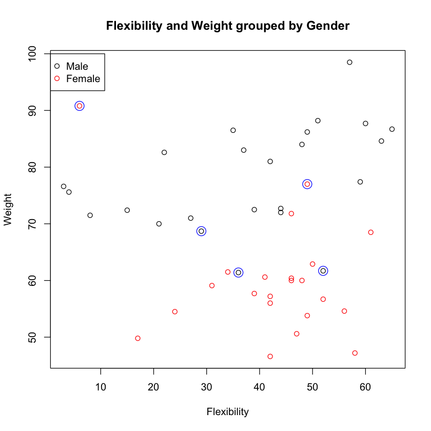
Who was predicted wrongly?
misses <- y.pred != y.test
df.test[misses,]
| ID | GENDER | FLEXPRE | BAWPRE | |
|---|---|---|---|---|
| 65 | 65 | Male | 29 | 68.7 |
| 77 | 77 | Male | 36 | 61.4 |
| 149 | 66 | Female | 6 | 90.8 |
| 21 | 21 | Male | 52 | 61.7 |
| 147 | 64 | Female | 49 | 77 |
plot(df.test$FLEXPRE, df.test$BAWPRE, col=df.test$GENDER,
     xlab="Flexibility", ylab="Weight",
     main="Flexibility and Weight grouped by Gender")
points(df.test$FLEXPRE[misses], df.test$BAWPRE[misses], col="blue", cex=2)

legend(0, 100, c("Male", "Female"), pch=1, col=1:2)
Work!
Repeat the analysis using the Bfppre and Fvcpre variables as predictors instead. Do you get better or worse predictions?
Q!. Extract the relevant variables into a new data frame.
Q2. Visualize Bfppre and Fvcpre grouped by gender.
Q3. Split the data into training and test data sets using a 2/3, 1/3 ratio.
Q4. Find the predictions make by knn with 5 neighbors.
Q5.. Make a table of true positives, false positives, true negatives and false negatives. Calculate
- accuracy
- sensitivity
- specificity
- possitive predicrvie value
- negative predictive value
- f-score (harmonic mean of senistivity and specificity)
Look up definitions in Wikipedia if you don’t know what these mean.
Q6 Make a plot to identify mis-classified subjects if any.
Cross-validation
Splitting into training and test data set is all well and good, but when the amound data we have is small, it is wastful to have 1/4 or 1/3 as “hold out” test data that is not used to train the algorithm. An alternaitve is to perform cross-validation, in which we split the data into k equal groups and cycle through all possible combinatinos of k-1 training and 1 test group. For example, if we split the data into 4 groups (“4-fold cross-validation”), we would do
- Train on 1,2,3 and Test on 4
- Train on 1,2,4 and Test on 3
- Train on 1,3,4 and Test on 2
- Train on 2,3,4 and Test on 1
then finally sum the test results to evalate the algorithm’s performance. The limiting example where we split into as many n groups (where n is the number of data poits) and test on only 1 data point each time is known as Leave-One-Out-Cross-Validation (LOOCV).
LOOCV
We will use a simple (inefficient) loop version of the algorithm that should be quite easy to understand.
First, we will recreat the data set in case you overwrote the variables in the exercises.
df <- healthdy[,c("ID", "GENDER", "FLEXPRE", "BAWPRE")]
df$ID <- factor(df$ID)
df$GENDER <- factor(df$GENDER, labels = c("Male", "Female"))
df$FLEXPRE <- as.numeric(df$FLEXPRE)
summary(df)
      ID         GENDER       FLEXPRE          BAWPRE
0      :  2   Male  : 82   Min.   : 1.00   Min.   :35.20
2      :  2   Female:100   1st Qu.:26.00   1st Qu.:57.73
3      :  2                Median :42.00   Median :65.05
4      :  2                Mean   :38.76   Mean   :66.99
5      :  2                3rd Qu.:52.00   3rd Qu.:74.50
6      :  2                Max.   :67.00   Max.   :98.50
(Other):170
y.test <- df[,"GENDER"]
y.pred <- y.test # we will overwirite the entries in the loop
for (i in 1:nrow(df)) {
    x.test <- df[i, c("FLEXPRE", "BAWPRE")]
    x.train <- df[-i, c("FLEXPRE", "BAWPRE")] # the minus menas keep all rows except i
    y.train <- df[-i, "GENDER"]
    y.pred[i] <- knn(x.train, x.test, cl=y.train, k=3)
}
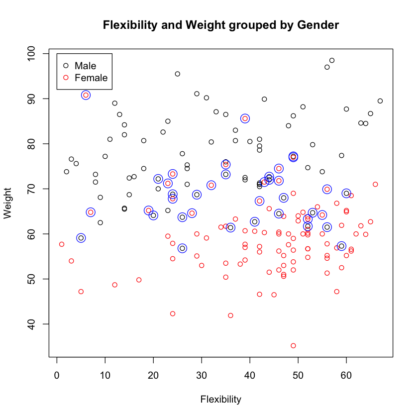
table(y.pred, y.test)
        y.test
y.pred   Male Female
  Male     62     18
  Female   20     82
misses <- y.test != y.pred

plot(df$FLEXPRE, df$BAWPRE, col=df$GENDER,
     xlab="Flexibility", ylab="Weight",
     main="Flexibility and Weight grouped by Gender")
points(df$FLEXPRE[misses], df$BAWPRE[misses], col="blue", cex=2)

legend(0, 100, c("Male", "Female"), pch=1, col=1:2)
Work!
Q1. Increase the number of neighbors to 7. Does it improve the reuslts? Whatt are the tradeoff of increasing or decraesaing the number of neighbors?
Q2. Implement 5-fold cross-validation for the FLEXPRE and BAWPRE variables. Tablutate the hits and misses and make a plot as in the previous examples.
Supervised Learning Continued - What Could Go Wrong?
In this lab, we will demonstrate some common pitfalls that may be encountered in performing a supervised learning analysis. To this end, we will simulate data under the null (meaning, we will simulate no relationship between outcome and independent variables) to observe situations where we may commit type I error.
## Supervised

# Simulate noisy data matrix (EXPRS)
set.seed(123)
# We'll use 2 groups of 20 subjects - think 20 cases and 20 controls
n=20
# Simulate 1000 genes
m=1000

# randomly generate a matrix of 'expression levels' -- any continuous variable we may be interested in
EXPRS=matrix(rnorm(2*n*m),2*n,m)

# Just naming rows and columns
rownames(EXPRS)=paste("patient",1:(2*n),sep="")
colnames(EXPRS)=paste("gene exp",1:m,sep="")

# The group labels are assigned arbitrarily - i.e. we are just randomly assigning
#                case/control status with no reference to gene expression
grp=rep(0:1,c(n,n))
#Pick the top 10 features based on the
#two-sample $t$-test

# load the library 'genefilter' - part of the Bioconductor suite
library(genefilter)

# rowttests is a genefilter function that performs a student t test on rows.

ttest.data=rowttests(t(EXPRS), factor(grp))
head(ttest.data)
| statistic | dm | p.value | |
|---|---|---|---|
| gene exp1 | 0.6746243 | 0.192881 | 0.5039985 |
| gene exp2 | 0.7417175 | 0.2264023 | 0.4628184 |
| gene exp3 | 3.025423 | 0.7344752 | 0.004436959 |
| gene exp4 | 0.4030939 | 0.1349871 | 0.6891382 |
| gene exp5 | 0.9545301 | 0.3004477 | 0.3458485 |
| gene exp6 | 0.3305064 | 0.09782354 | 0.7428327 |
# Extract the absolute value of the statistic
stats=abs(ttest.data$statistic)

# 'order' will return the indices of ascending values of it's argument
ii=order(-stats)

#Filter out all genes (i.e. columns of the matrix) except the top 10 rated by stats

TOPEXPRS=EXPRS[, ii[1:10]]
dim(TOPEXPRS)
- 40
- 10
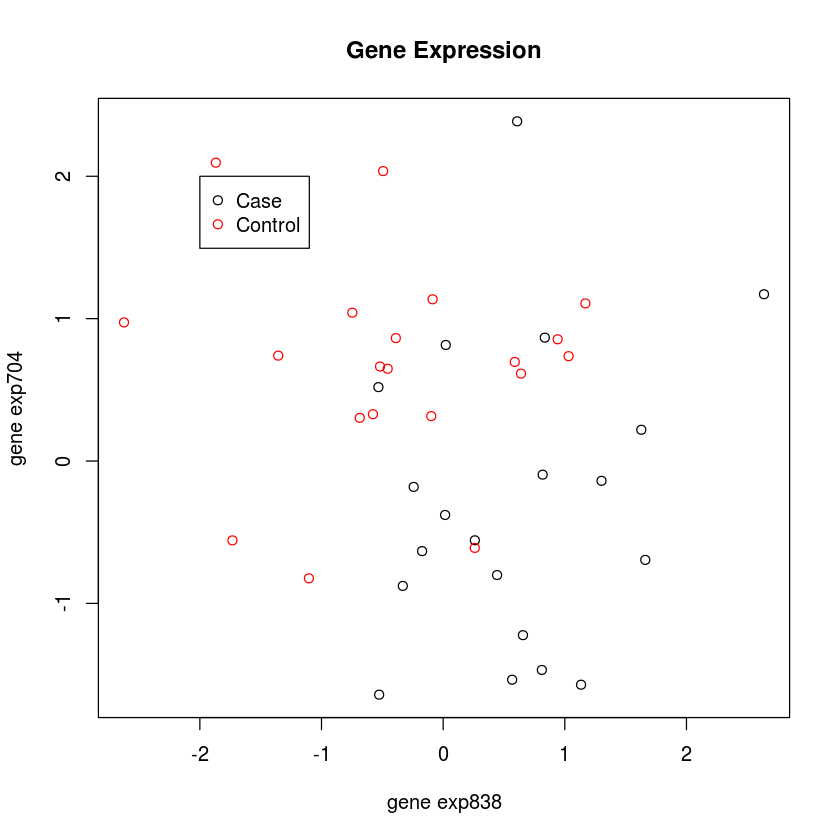
Now we will perform a 3-nearest-neighbor clustering, just like we did with the health dynamics class data.
plot(TOPEXPRS, col=grp+1,
      main="Gene Expression")
legend(-2, 2, c("Case", "Control"), pch=1, col=1:2)
# Fit 3-NN
library(class)
mod0=knn(train=TOPEXPRS,test=TOPEXPRS,cl=grp,k=3)
print(mod0)

# Error Resubstituion
table(mod0,grp)
 [1] 0 0 1 0 0 0 0 0 0 0 0 0 0 1 0 0 0 0 0 1 1 1 1 1 1 1 1 1 1 1 1 1 1 1 1 1 1 1
[39] 1 1
Levels: 0 1
    grp
mod0  0  1
   0 17  0
   1  3 20
# Naive CV
mod1=knn.cv(TOPEXPRS,grp,k=3)
table(mod1,grp)
    grp
mod1  0  1
   0 16  0
   1  4 20
This looks like differential gene expression. We can accurately predict case-control status, based on gene expression. But, we haven’t cross-validated. And we have only 40 subjects and have looked at 1000 genes! Let’s do it the right way now. This is like tossing a coin 40 times, and repeating that 1000 times. We will see some very long strings of heads and tails in some replicates - just by chance!
# Oh! Super fancy code! I'll rewrite if there is time. Otherwise, we need to skip through.

# Proper CV
top.features=function(EXP,resp,test,fsnum)
  {
    top.features.i=function(i,EXP,resp,test,fsnum)
      {
        stats=abs(mt.teststat(EXP[,-i],resp[-i],test=test))
        ii=order(-stats)[1:fsnum]
        rownames(EXP)[ii]
      }
    sapply(1:ncol(EXP),top.features.i,EXP=EXP,resp=resp,test=test,fsnum=fsnum)
  }
# This function evaluates the knn

knn.loocv=function(EXP,resp,test,k,fsnum,tabulate=FALSE,permute=FALSE)
  {
    if(permute)
      resp=sample(resp)
    topfeat=top.features(EXP,resp,test,fsnum)
    pids=rownames(EXP)
    EXP=t(EXP)
    colnames(EXP)=as.character(pids)
    knn.loocv.i=function(i,EXP,resp,k,topfeat)
      {
        ii=topfeat[,i]
        mod=knn(train=EXP[-i,ii],test=EXP[i,ii],cl=resp[-i],k=k)[1]
      }
    out=sapply(1:nrow(EXP),knn.loocv.i,EXP=EXP,resp=resp,k=k,topfeat=topfeat)
    if(tabulate)
      out=ftable(pred=out,obs=resp)
    return(out)
}
library(multtest)
knn.loocv(t(EXPRS),as.integer(grp),"t.equalvar",3,10,TRUE)
Loading required package: Biobase
Loading required package: BiocGenerics
Loading required package: parallel

Attaching package: ‘BiocGenerics’

The following objects are masked from ‘package:parallel’:

    clusterApply, clusterApplyLB, clusterCall, clusterEvalQ,
    clusterExport, clusterMap, parApply, parCapply, parLapply,
    parLapplyLB, parRapply, parSapply, parSapplyLB

The following object is masked from ‘package:stats’:

    xtabs

The following objects are masked from ‘package:base’:

    anyDuplicated, append, as.data.frame, as.vector, cbind, colnames,
    do.call, duplicated, eval, evalq, Filter, Find, get, intersect,
    is.unsorted, lapply, Map, mapply, match, mget, order, paste, pmax,
    pmax.int, pmin, pmin.int, Position, rank, rbind, Reduce, rep.int,
    rownames, sapply, setdiff, sort, table, tapply, union, unique,
    unlist

Welcome to Bioconductor

    Vignettes contain introductory material; view with
    'browseVignettes()'. To cite Bioconductor, see
    'citation("Biobase")', and for packages 'citation("pkgname")'.
     obs  0  1
pred
0         7  7
1        13 13
Well, now that looks right! We are no longer fitting noise. What’s the difference? Everytime we perform a validation step, we need to re-evaluate the top ten picks!