Coding Exercises
Practice 1
- Create a sequence of integers starting from 12 and ending at 17.
12:17
[1] 12 13 14 15 16 17
- Create a vector of length 10 starting from \(\pi\) and ending at \(2\pi\) with evenly spaced intervals between numbers.
seq(pi, 2*pi, length.out = 10)
[1] 3.141593 3.490659 3.839724 4.188790 4.537856 4.886922 5.235988 5.585054
[9] 5.934119 6.283185
- Find the sum of all numbers between 1 and 1000 that are divisible by 3.
ns <- 1:1000
idx <- ns %% 3 == 0
sum(ns[idx])
[1] 166833
- Find the sum of the square numbers (e.g. 1, 4, 9, 16, ...) from 1 that are less than or equal to 10,000.
top <- sqrt(10000)
ns <- 1:top
sum(ns^2)
[1] 338350
Loop through the numbers from 1 to 20. If the number is divisible by 3, print “Fizz”. If the number is divisible by 5, print “Buzz”. If it is divisible by both 3 and 5 print “FizzBuzz”. Otherwise just print the number. Your output should look something like
1
2
Fizz
4
Buzz
...
for (i in 1:20) {
    if (i %% 15 == 0)
        print("FizzBuzz")
    else if (i %% 3 == 0)
        print("Fizz")
    else if (i %% 5 == 0)
        print("Buzz")
    else print(i)
}
[1] 1
[1] 2
[1] "Fizz"
[1] 4
[1] "Buzz"
[1] "Fizz"
[1] 7
[1] 8
[1] "Fizz"
[1] "Buzz"
[1] 11
[1] "Fizz"
[1] 13
[1] 14
[1] "FizzBuzz"
[1] 16
[1] 17
[1] "Fizz"
[1] 19
[1] "Buzz"
- Generate 1000 numbers from the standard normal distirbution. How many of these numbers are greater than 0?
xs <- rnorm(1000)
sum(xs > 0)
[1] 503
Start by copying and pasting the code below in a Code cell
set.seed(123)
n <- 10
case <- rnorm(n, 0, 1)
ctrl <- rnorm(n, 0.1, 1)
Run the above code, then state the null hypothesis for comparing the mean between cases and controls. Perform a t-test with \(n = 10\) and $n = \(1000\).
set.seed(123)
n <- 10
case <- rnorm(n, 0, 1)
ctrl <- rnorm(n, 0.1, 1)

t.test(case, ctrl)
    Welch Two Sample t-test

data:  case and ctrl
t = -0.5249, df = 17.872, p-value = 0.6061
alternative hypothesis: true difference in means is not equal to 0
95 percent confidence interval:
 -1.1710488  0.7030562
sample estimates:
 mean of x  mean of y
0.07462564 0.30862196
set.seed(123)
n <- 1000
case <- rnorm(n, 0, 1)
ctrl <- rnorm(n, 0.1, 1)

t.test(case, ctrl)
    Welch Two Sample t-test

data:  case and ctrl
t = -2.8229, df = 1997.355, p-value = 0.004806
alternative hypothesis: true difference in means is not equal to 0
95 percent confidence interval:
 -0.2141064 -0.0385684
sample estimates:
 mean of x  mean of y
0.01612787 0.14246525
- You are plannning an experiment to test the effect of a new drug on mouse growth as measured in grams. You plan to give the drug to a treatment group and not to an otherwise identical control group. You consider differences to be meaningful if the mean weights differ by at least 10 grams. From previous experiments, you know that the standard deviation between mice weights is 20 grams. What sample size do you need in each group for 80%, 90% and 100% power (use p=0.05)? If you recorded weights in kilograms instead, would the sample sizes need to change?
library(pwr)
pwr.t.test(d = 10/20, sig.level = 0.05, power = 0.8, type = "two.sample")
     Two-sample t test power calculation

              n = 63.76561
              d = 0.5
      sig.level = 0.05
          power = 0.8
    alternative = two.sided

NOTE: n is number in each group
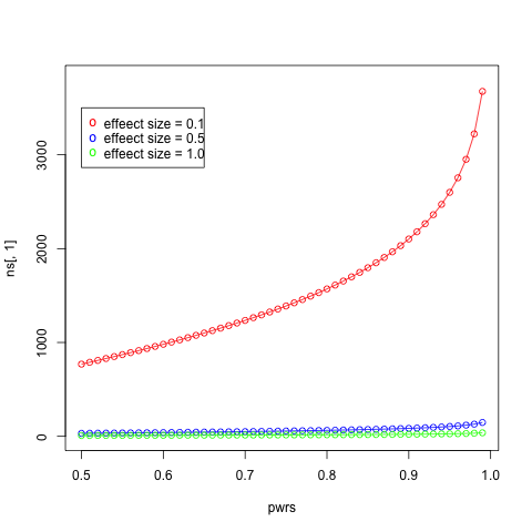
- Make a plot of sample size (y-axis) against power (x-axis) for powers ranging from 0.01 to 0.99 in steps of 0.01 with an effect size of 0.1. Add in curves of different colors for effect sizes of 0.5 and 1.0. Add a legend for each curve.
ans <- pwr.t.test(d = 10/20, sig.level = 0.05, power = 0.8, type = "two.sample")
ans$n
[1] 63.76561
pwrs <- seq(0.5, 0.99, by=0.01)
ds <- c(0.1, 0.5, 1.0)
nrow <- length(pwrs)
ncol <- length(ds)
ns <- matrix(, nrow=nrow, ncol=ncol)
for (i in 1:nrow) {
    for (j in 1:ncol) {
        ns[i, j] <- pwr.t.test(d = ds[j], sig.level = 0.05, power = pwrs[i], type = "two.sample")$n
    }
}
plot(pwrs, ns[,1], type='o', col="red", ylim = c(0, 3800))
lines(pwrs, ns[,2], type='o', col="blue")
lines(pwrs, ns[,3], type='o', col="green")
legend(0.5, 3500, paste("effeect size =", c("0.1", "0.5", "1.0")), col=c("red", "blue", "green"), pch="o")
- Calcualte the probabity that you will see the sequence H, H, H, H when you toss a coin 4 times (on pen and paper!). Now conduct 10,000 simulation experiments in which you perform 4 coin tosses per experiment and record the number of heads. What is the frequency of all heads and is this similar to what you calculated?
0.5^4
[1] 0.0625
expts <- rbinom(10000, size=4, prob=0.5)
sum(expts == 4)
[1] 613
- The
anscombedataframe has 8 columns and 11 rows. Perform a linear regression of \(y1\) against \(x1\), \(y2\) against \(x2\) and so on and report what the intercept and slope are in each case (Note: the anscombe dataframe is already loaded).
model <- lm(y1 ~ x1, data=anscombe)
model$coefficients
(Intercept)          x1
  3.0000909   0.5000909
model <- lm(y2 ~ x2, data=anscombe)
model$coefficients
model <- lm(y3 ~ x3, data=anscombe)
model$coefficients
model <- lm(y4 ~ x4, data=anscombe)
model$coefficients
(Intercept)          x4
  3.0017273   0.4999091
- Now plot four scatter plots, one for \(y1\) against x1$, \(y2\) against \(x2\) and so on for the same anscombe datafraem.
par(mfrow=c(2,2))
with(anscombe, plot(x1, y1, type="p"))
with(anscombe, plot(x2, y2, type="p"))
with(anscombe, plot(x3, y3, type="p"))
with(anscombe, plot(x4, y4, type="p"))

- Write a function that takes two p-dimensional vectors and retunrs the Euclidean distance between them. The definitiion for Euclidean distance in p dimensions extneds the 2-dimensional definition in the obvious way. For example, the distance between the 3-dimensonal vectors \((1,2,3)\) and \((2,4,6)\) is \(\sqrt{((1-2)^2 + (2-4)^2 + (3-6)^2)}\).
my.dist <- function(v1, v2) {
    return(sqrt(sum((v1-v2)^2)))
}

my.dist(c(0,0), c(3,4))
[1] 5
- Write a function to calculate the median of a vector of numbers. Recall that if the vector is of odd length, the median is the central number of the sorted vacotr; othersise it is the average of the two central numbers.
my.median <- function(v) {
    v <- sort(v)
    n <- length(v)
    if (n %% 2 == 1)
        ans <- v[floor(n/2)]
    else {
        low <- floor(n/2)
        ans <- mean(v[low:(low+1)])
    }
    return(ans)
}
my.median(1:11)
[1] 5
my.median(1:12)
[1] 6.5
- Write a function called
peekthat will take a dataframe and a number as arguments - so you would eovke the function with a call likepeek(df, n). What this function does is return \(n\) rows at random (no duplicate rows). If \(n\) is greater than the number of rows, the enitre data frame is returned.
peek <- function(df, n) {
    if (n > length(df)) {
        ans <- df
    }
    else {
        idx <- sample(1:length(df), n, replace=FALSE)
        ans <- df[idx,]
    }
    return(ans)
}
peek(anscombe, 3)
  x1 x2 x3 x4   y1   y2    y3   y4
4  9  9  9  8 8.81 8.77  7.11 8.84
3 13 13 13  8 7.58 8.74 12.74 7.71
5 11 11 11  8 8.33 9.26  7.81 8.47
Practice 2
Working with dataframes
Practice TWO is meant to help you get comfortable working with data frames, and the basic ways you can slice and dice datafrmaes.
- How many rows and columns are there in the
mtcarsdataframe?
(nrow(mtcars))
(ncol(mtcars))
[1] 32
[1] 11
dim(mtcars)
[1] 32 11
- Show the last 6 rows of
mtcars.
tail(mtcars, 6)
                mpg cyl  disp  hp drat    wt qsec vs am gear carb
Porsche 914-2  26.0   4 120.3  91 4.43 2.140 16.7  0  1    5    2
Lotus Europa   30.4   4  95.1 113 3.77 1.513 16.9  1  1    5    2
Ford Pantera L 15.8   8 351.0 264 4.22 3.170 14.5  0  1    5    4
Ferrari Dino   19.7   6 145.0 175 3.62 2.770 15.5  0  1    5    6
Maserati Bora  15.0   8 301.0 335 3.54 3.570 14.6  0  1    5    8
Volvo 142E     21.4   4 121.0 109 4.11 2.780 18.6  1  1    4    2
- Show 6 rows at random (no duplicates) from
mtcars
ridx <- sample(1:nrow(mtcars), 6, replace=FALSE)
mtcars[ridx,]
               mpg cyl  disp  hp drat    wt  qsec vs am gear carb
Toyota Corona 21.5   4 120.1  97 3.70 2.465 20.01  1  0    3    1
Camaro Z28    13.3   8 350.0 245 3.73 3.840 15.41  0  0    3    4
Valiant       18.1   6 225.0 105 2.76 3.460 20.22  1  0    3    1
Merc 280C     17.8   6 167.6 123 3.92 3.440 18.90  1  0    4    4
Fiat 128      32.4   4  78.7  66 4.08 2.200 19.47  1  1    4    1
AMC Javelin   15.2   8 304.0 150 3.15 3.435 17.30  0  0    3    2
- Display information only for the subset of cars with automatic transmission.
mtcars[mtcars$am == 1,]
                mpg cyl  disp  hp drat    wt  qsec vs am gear carb
Mazda RX4      21.0   6 160.0 110 3.90 2.620 16.46  0  1    4    4
Mazda RX4 Wag  21.0   6 160.0 110 3.90 2.875 17.02  0  1    4    4
Datsun 710     22.8   4 108.0  93 3.85 2.320 18.61  1  1    4    1
Fiat 128       32.4   4  78.7  66 4.08 2.200 19.47  1  1    4    1
Honda Civic    30.4   4  75.7  52 4.93 1.615 18.52  1  1    4    2
Toyota Corolla 33.9   4  71.1  65 4.22 1.835 19.90  1  1    4    1
Fiat X1-9      27.3   4  79.0  66 4.08 1.935 18.90  1  1    4    1
Porsche 914-2  26.0   4 120.3  91 4.43 2.140 16.70  0  1    5    2
Lotus Europa   30.4   4  95.1 113 3.77 1.513 16.90  1  1    5    2
Ford Pantera L 15.8   8 351.0 264 4.22 3.170 14.50  0  1    5    4
Ferrari Dino   19.7   6 145.0 175 3.62 2.770 15.50  0  1    5    6
Maserati Bora  15.0   8 301.0 335 3.54 3.570 14.60  0  1    5    8
Volvo 142E     21.4   4 121.0 109 4.11 2.780 18.60  1  1    4    2
- Display information only for the subset of cars with weight between 2 and 3.
mtcars[(2 < mtcars$wt) & (mtcars$wt < 3),]
               mpg cyl  disp  hp drat    wt  qsec vs am gear carb
Mazda RX4     21.0   6 160.0 110 3.90 2.620 16.46  0  1    4    4
Mazda RX4 Wag 21.0   6 160.0 110 3.90 2.875 17.02  0  1    4    4
Datsun 710    22.8   4 108.0  93 3.85 2.320 18.61  1  1    4    1
Fiat 128      32.4   4  78.7  66 4.08 2.200 19.47  1  1    4    1
Toyota Corona 21.5   4 120.1  97 3.70 2.465 20.01  1  0    3    1
Porsche 914-2 26.0   4 120.3  91 4.43 2.140 16.70  0  1    5    2
Ferrari Dino  19.7   6 145.0 175 3.62 2.770 15.50  0  1    5    6
Volvo 142E    21.4   4 121.0 109 4.11 2.780 18.60  1  1    4    2
- What is the mean weight of all cars?
mean(mtcars$wt)
[1] 3.21725
(7) What is the mean weight of cars wtih `mpg` greater than 20?
mean(mtcars[mtcars$mpg > 20, "wt"])
[1] 2.418071
- Add a column
kplshowing the number of kilometers per liter (1 mile = 1.609344 kilometers, and 1 gallon = 3.78541178 liters)
mpg.to.kpl <- function(mpg) {
    return(mpg * 1.609344 / 3.78541178)
}
mtcars$kpl <- mpg.to.kpl(mtcars$mpg)
head(mtcars)
                   mpg cyl disp  hp drat    wt  qsec vs am gear carb      kpl
Mazda RX4         21.0   6  160 110 3.90 2.620 16.46  0  1    4    4 8.928018
Mazda RX4 Wag     21.0   6  160 110 3.90 2.875 17.02  0  1    4    4 8.928018
Datsun 710        22.8   4  108  93 3.85 2.320 18.61  1  1    4    1 9.693277
Hornet 4 Drive    21.4   6  258 110 3.08 3.215 19.44  1  0    3    1 9.098075
Hornet Sportabout 18.7   8  360 175 3.15 3.440 17.02  0  0    3    2 7.950187
Valiant           18.1   6  225 105 2.76 3.460 20.22  1  0    3    1 7.695101
- Make a new dataframe
mtcars.1with only thempgandkplcolumns.
mtcars.1 <- mtcars[, c("mpg", "kpl")]
head(mtcars.1)
                   mpg      kpl
Mazda RX4         21.0 8.928018
Mazda RX4 Wag     21.0 8.928018
Datsun 710        22.8 9.693277
Hornet 4 Drive    21.4 9.098075
Hornet Sportabout 18.7 7.950187
Valiant           18.1 7.695101
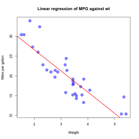
- Perform a linear regression model of
mpgagainstwt. Plot the model fit.
fit <- lm(mpg ~ wt, data=mtcars)
summary(fit)
Call:
lm(formula = mpg ~ wt, data = mtcars)

Residuals:
    Min      1Q  Median      3Q     Max
-4.5432 -2.3647 -0.1252  1.4096  6.8727

Coefficients:
            Estimate Std. Error t value Pr(>|t|)
(Intercept)  37.2851     1.8776  19.858  < 2e-16 *
wt           -5.3445     0.5591  -9.559 1.29e-10 *
---
Signif. codes:  0 ‘*’ 0.001 ‘’ 0.01 ‘*’ 0.05 ‘.’ 0.1 ‘ ’ 1

Residual standard error: 3.046 on 30 degrees of freedom
Multiple R-squared:  0.7528,        Adjusted R-squared:  0.7446
F-statistic: 91.38 on 1 and 30 DF,  p-value: 1.294e-10
plot(mtcars$wt, mtcars$mpg, col=rgb(0,0,1,0.5), pch=16, cex=2.0,
    xlab="Weigth", ylab="Miles per gallon",
     main="Linear regression of MPG against wt")
abline(fit, col="red", lwd=2)
- Print 10 rows at ranodm from the
irisdataframe
ridx <- sample(1:nrow(iris), 10, replace = FALSE)
iris[ridx,]
    Sepal.Length Sepal.Width Petal.Length Petal.Width    Species
136          7.7         3.0          6.1         2.3  virginica
10           4.9         3.1          1.5         0.1     setosa
29           5.2         3.4          1.4         0.2     setosa
80           5.7         2.6          3.5         1.0 versicolor
54           5.5         2.3          4.0         1.3 versicolor
11           5.4         3.7          1.5         0.2     setosa
58           4.9         2.4          3.3         1.0 versicolor
56           5.7         2.8          4.5         1.3 versicolor
150          5.9         3.0          5.1         1.8  virginica
59           6.6         2.9          4.6         1.3 versicolor
- Find the mean Sepal.Length Sepal.Width Petal.Length Petal.Width for
each iris species using the
aggregatecommand.
aggregate(iris[,1:4], by=list(iris$Species), FUN=mean)
     Group.1 Sepal.Length Sepal.Width Petal.Length Petal.Width
1     setosa        5.006       3.428        1.462       0.246
2 versicolor        5.936       2.770        4.260       1.326
3  virginica        6.588       2.974        5.552       2.026
Practice 3
- Make a plot of the standard normal curve on the interval [-4, 4]. Give the plot a title “Standard normal curve”, an x label of “Normal deviate” and a y label of “Density”.
x <- pretty(-4:4, n=100)
y <- dnorm(x)
plot(x, y, type="l", main="Standard normal curve", xlab="Normal deviate", ylab="Density")

- What is the area under the curve to the right of x=3? In other words, what is the probability of drawing a random number from the normal distribution that is 3 standard deviations or more larger than the mean?
1 - pnorm(3)
- If the expression valuse for a gene are normally distributed with mean 10 and standard deviation 2, what is the value of a gene at the 95th percentile?
qnorm(0.95, mean=10, sd=2)
Generate 50 numbers from a normal distribtuion with mean=10 and sd=2. Now trnaform this vector so that the numbers have a stnadard normal distribtuion with mean=0 and sd=1.
x <- rnorm(50, 10, 2)
z <- (x - mean(x))/sd(x)
- A t-test with 6 degrees of freedom has a score of 3.5. Using only the dt, pt, qt or rt probability functions, what is the p-value if this was a two-sided test? Recall that a p-value is the probailty of seeing a value as extreme or more extreme than the observed score, assuming the score was drawn from the specified distirbution.
2*(1 - pt(3.5, df = 6))
- Draw 1 million random numbers from the t-distirbution with 6 degrees of freedom. How many times is the numbr less than -3.5 or greater than 3.5?
x <- rt(100000, df=6)
sum(abs(x) > 3.5)
- Find the mean value of all numeric variables for the mtcars data, grouping by number of gears and automtatic or manual transmission. (Hint: Use the aggregate function)
with(mtcars, aggregate(mtcars, by=list(gear=gear, transmission=am), FUN=mean))
| gear | transmission | mpg | cyl | disp | hp | drat | wt | qsec | vs | am | gear | carb | |
|---|---|---|---|---|---|---|---|---|---|---|---|---|---|
| 1 | 3 | 0 | 16.10667 | 7.466667 | 326.3 | 176.1333 | 3.132667 | 3.8926 | 17.692 | 0.2 | 0 | 3 | 2.666667 |
| 2 | 4 | 0 | 21.05 | 5 | 155.675 | 100.75 | 3.8625 | 3.305 | 20.025 | 1 | 0 | 4 | 3 |
| 3 | 4 | 1 | 26.275 | 4.5 | 106.6875 | 83.875 | 4.13375 | 2.2725 | 18.435 | 0.75 | 1 | 4 | 2 |
| 4 | 5 | 1 | 21.38 | 6 | 202.48 | 195.6 | 3.916 | 2.6326 | 15.64 | 0.2 | 1 | 5 | 4.4 |
library(plyr)
library(reshape2)
data(airquality)
Warning message:
: package ‘plyr’ was built under R version 3.1.3
head(airquality)
| Ozone | Solar.R | Wind | Temp | Month | Day | |
|---|---|---|---|---|---|---|
| 1 | 41 | 190 | 7.4 | 67 | 5 | 1 |
| 2 | 36 | 118 | 8 | 72 | 5 | 2 |
| 3 | 12 | 149 | 12.6 | 74 | 5 | 3 |
| 4 | 18 | 313 | 11.5 | 62 | 5 | 4 |
| 5 | NA | NA | 14.3 | 56 | 5 | 5 |
| 6 | 28 | NA | 14.9 | 66 | 5 | 6 |
- Use
meltto convert the airquality dataframe into a “tall” format using Month and Day as teh id variables, saving it as a new datafrmae. Print the first 6 rows.
md <- melt(airquality, id=c("Month", "Day"))
head(md)
| Month | Day | variable | value | |
|---|---|---|---|---|
| 1 | 5 | 1 | Ozone | 41 |
| 2 | 5 | 2 | Ozone | 36 |
| 3 | 5 | 3 | Ozone | 12 |
| 4 | 5 | 4 | Ozone | 18 |
| 5 | 5 | 5 | Ozone | NA |
| 6 | 5 | 6 | Ozone | 28 |
- Find the avarage values of Ozone, Solar.R, Wind and Temp for each
month using
dcast. Hint: Give an extra argumentna.rm = TRUEto ignore missing data.
dcast(md, Month ~ variable, mean, na.rm = TRUE)
| Month | Ozone | Solar.R | Wind | Temp | |
|---|---|---|---|---|---|
| 1 | 5 | 23.61538 | 181.2963 | 11.62258 | 65.54839 |
| 2 | 6 | 29.44444 | 190.1667 | 10.26667 | 79.1 |
| 3 | 7 | 59.11538 | 216.4839 | 8.941935 | 83.90323 |
| 4 | 8 | 59.96154 | 171.8571 | 8.793548 | 83.96774 |
| 5 | 9 | 31.44828 | 167.4333 | 10.18 | 76.9 |
- Find the avarage values of Ozone, Solar.R, Wind and Temp for each
month using
dcast, but only for the first 2 weeks of each month. Hint: Give an extra argumentna.rm = TRUEto ignore missing data. Hint: Use the subset argument.
dcast(md, Month ~ variable, mean, subset = .(Day < 15), na.rm = TRUE)
| Month | Ozone | Solar.R | Wind | Temp | |
|---|---|---|---|---|---|
| 1 | 5 | 19.41667 | 200.0909 | 11.17857 | 66.28571 |
| 2 | 6 | 40.5 | 249.1429 | 10.73571 | 82.85714 |
| 3 | 7 | 64.81818 | 228.7143 | 9.007143 | 84.85714 |
| 4 | 8 | 58.41667 | 168.7273 | 8.721429 | 85.5 |
| 5 | 9 | 43.35714 | 188.6429 | 9.407143 | 82.21429 |
Questions below use the day.1 and day.2 dataframes
set.seed(123)
pid.1 <- c(1,1,2,2)
gid.1 <- c(1,2,1,2)
val.1 <- rnorm(4)
day.1 <- data.frame(pid=pid.1, gid=gid.1, val=val.1)

pid.2 <- c(1,1,2,2)
gid.2 <- c(1,2,1,2)
val.2 <- 1 + rnorm(4)
day.2 <- data.frame(pid=pid.2, gid=gid.2, val=val.2)
day.1
| pid | gid | val | |
|---|---|---|---|
| 1 | 1 | 1 | -0.5604756 |
| 2 | 1 | 2 | -0.2301775 |
| 3 | 2 | 1 | 1.558708 |
| 4 | 2 | 2 | 0.07050839 |
day.2
| pid | gid | val | |
|---|---|---|---|
| 1 | 1 | 1 | 1.129288 |
| 2 | 1 | 2 | 2.715065 |
| 3 | 2 | 1 | 1.460916 |
| 4 | 2 | 2 | -0.2650612 |
- Suppose day.1 and day.2 are results from experiments performed on
differnet days. Merge the data from day.1 and day.2 into a single
dataframe caleld
daysto combine the data sets.
days <- merge(day.1, day.2, by=c("pid", "gid"), suffixes = 1:2)
days
| pid | gid | val1 | val2 | |
|---|---|---|---|---|
| 1 | 1 | 1 | -0.5604756 | 1.129288 |
| 2 | 1 | 2 | -0.2301775 | 2.715065 |
| 3 | 2 | 1 | 1.558708 | 1.460916 |
| 4 | 2 | 2 | 0.07050839 | -0.2650612 |
- Sort the
daysdataframe by val1 in decreasing order.
days[order(-days$val1),]
| pid | gid | val1 | val2 | |
|---|---|---|---|---|
| 3 | 2 | 1 | 1.558708 | 1.460916 |
| 4 | 2 | 2 | 0.07050839 | -0.2650612 |
| 2 | 1 | 2 | -0.2301775 | 2.715065 |
| 1 | 1 | 1 | -0.5604756 | 1.129288 |
(12) Remove duplicate rows from the following dataframe.
df <- read.csv("df.csv")
df
| pid | gid | val1 | val2 | |
|---|---|---|---|---|
| 1 | 1 | 1 | -0.5604756 | 1.129288 |
| 2 | 1 | 1 | -0.5604756 | 1.129288 |
| 3 | 1 | 2 | -0.2301775 | 2.715065 |
| 4 | 2 | 2 | 0.07050839 | -0.2650612 |
| 5 | 2 | 2 | 0.07050839 | -0.2650612 |
| 6 | 2 | 1 | 1.558708 | 1.460916 |
unique(df)
| pid | gid | val1 | val2 | |
|---|---|---|---|---|
| 1 | 1 | 1 | -0.5604756 | 1.129288 |
| 3 | 1 | 2 | -0.2301775 | 2.715065 |
| 4 | 2 | 2 | 0.07050839 | -0.2650612 |
| 6 | 2 | 1 | 1.558708 | 1.460916 |
Practice 4
library(ggplot2)
library(reshape2)
library(pheatmap)
library(genefilter) # for rowttests
library(nlme)
data(Rail)
Attaching package: ‘genefilter’

The following object is masked from ‘package:base’:

    anyNA
Exericse 0
Using base graphics, make a 2 x 2 grid for plotting.
Top left - Generate 100 random numbers from a t-distribution with 5
degrees of freedom - Plot a normalized histogram (i.e. area sums to 1)
with 8 breaks - Overlay a smoothed density estimate (using density)
in orange - Overlay the true density estimate (using dt) in red -
Add a rug
Tor right - Using the iris data set, make a scatter plot of Sepal
length agaisnt Sepal width. Color the points by Species. - Add your own
title and x and y lables
Bottom left - Generate 100 numbers from a Poisson distribution with rate = 3 - Plot a bar chart showing the counts for each value
Bottom right - Make a box and whiskers plot of the 4 numeric variables
in the iris data set - Show vertical labels for all Species names -
Adjust the margins so that the labels are visible using the mar
(bottom, left, top, right) parameter. You can see the default values
with par()$mar. Remember to restore the orignal parameters at the
end.
Save the plot as a Portable Neetwork Graphics (png) file.
png("myplot.png")
par(mfrow=c(2,2))
x <- rt(100, df=5)
hist(x, breaks = 8, probability = TRUE)
lines(density(x), col="orange")
xp <- seq(min(x), max(x), length.out = 50)
lines(xp, dt(xp, df=5), col="red")
rug(x)
plot(iris$Sepal.Width, iris$Sepal.Length, col=iris$Species,
     main="Scatter by Iris species", ylab="Length", xlab="Width")
n <- rpois(100, lambda = 3)
barplot(table(n))
orig <- par(no.readonly=TRUE)
par(mar=c(6.1,4.1,4.1,2.1))
boxplot(iris[,1:4], las=2)
par(orig)
dev.off()
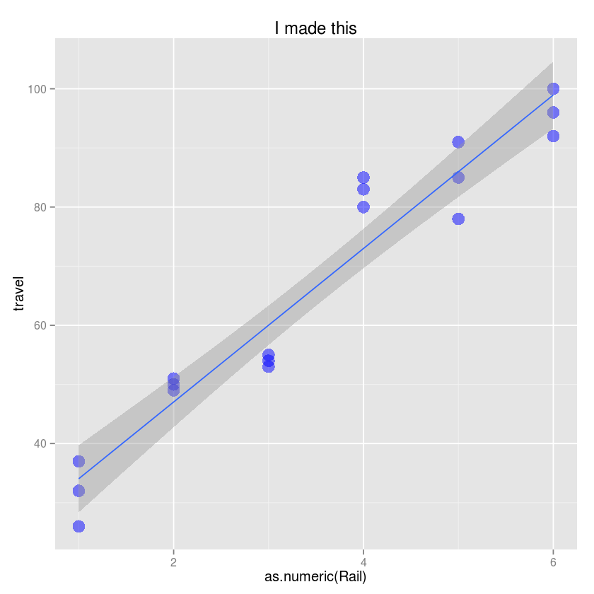
head(Rail)
| Rail | travel | |
|---|---|---|
| 1 | 1 | 55 |
| 2 | 1 | 53 |
| 3 | 1 | 54 |
| 4 | 2 | 26 |
| 5 | 2 | 37 |
| 6 | 2 | 32 |
Exercise 1
- Use the ggplot function
- Create a scatter plot with Rail on the x-axis and travel on the y-axis.
- CHange the title to “I made this!”
- Change the y-axis label to be “Zero-force travel time (nano-seconds)”
- Change the size of the points to 5
- Change the color of potins to blue and transparency to 0.5
- Add a simple linear regression line to the plot with 90% confidence intervals
ggplot(Rail, aes(x=as.numeric(Rail), y=travel)) +
geom_point(size=5, color="blue", alpha=0.5) +
geom_smooth(method="lm") +
labs(title="I made this", ylab="Zero-force travel time (nano-seconds)")
Exercise 2
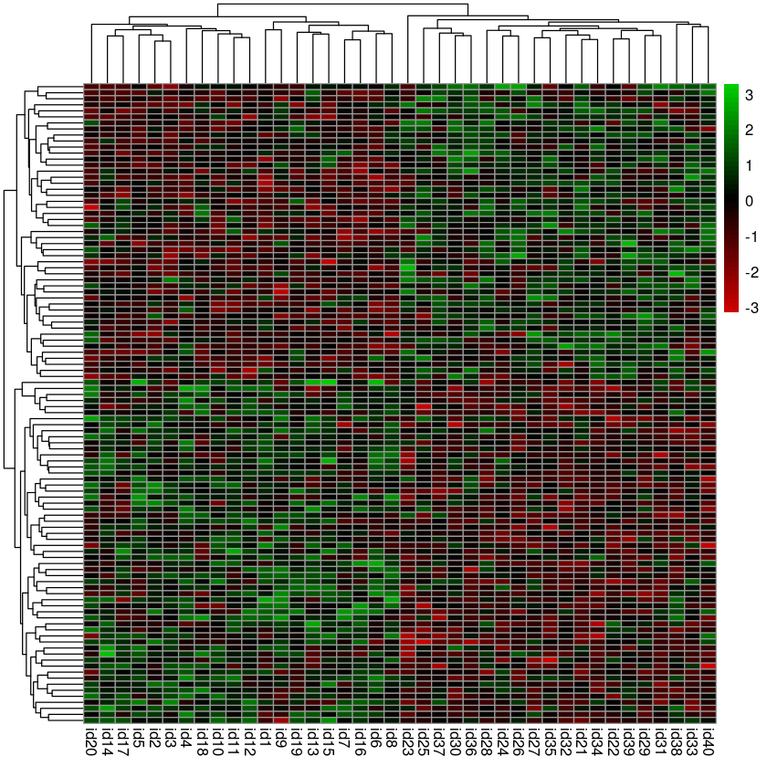
Here we will try to replicate the noise discovery heatmaps shown in the statistics class.
set.seed(123)

n <- 20 # number of subjects
m <- 20000 # number of genes
alpha <- 0.005 # significance level

# create a matrix of gene expression values with m rows and 2*n columns
M <- matrix(rnorm(2*n*m), m, 2*n)

# give row and column names
rownames(M) <- paste("G", 1:m, sep="")
colnames(M) <- paste("id", 1:(2*n), sep="")

# assign subjects inot equal sized groups
grp <- factor(rep(0:1, c(n, n)))

# calculate p-value using t-test for mean experession value of each gene
pvals <- rowttests(M, grp)$p.value

# extract the genes which meet the specified significance level
hits <- M[pvals < alpha,]
- Use pheatmap to plot a heatmap
- Remove the row names (Use tAB or R’s built-in help to figure out to do this)
- Use this color palette to map expression values to a red-blakc-green
scale
colorRampPalette(c("red3", "black", "green3"))(50)
pheatmap(hits, show_rownames = FALSE, color = colorRampPalette(c("red3", "black", "green3"))(50))
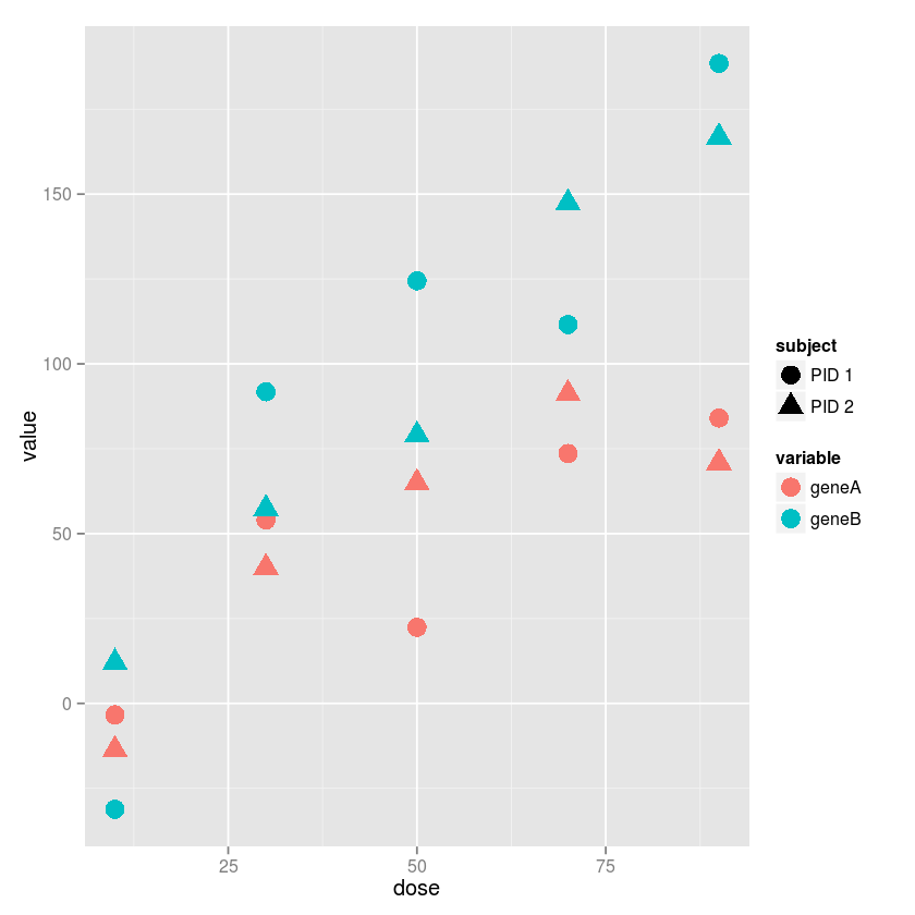
a1 <- 1
a2 <- 2
sigma1 <- 25
sigma2 <- 25
subject <- paste("PID", rep(1:2, each=5))
dose <- rep(seq(10, 100, 20), 2)
geneA <- a1 * dose + rnorm(length(dose), sd=sigma1)
geneB <- a2 * dose + rnorm(length(dose), sd=sigma2)
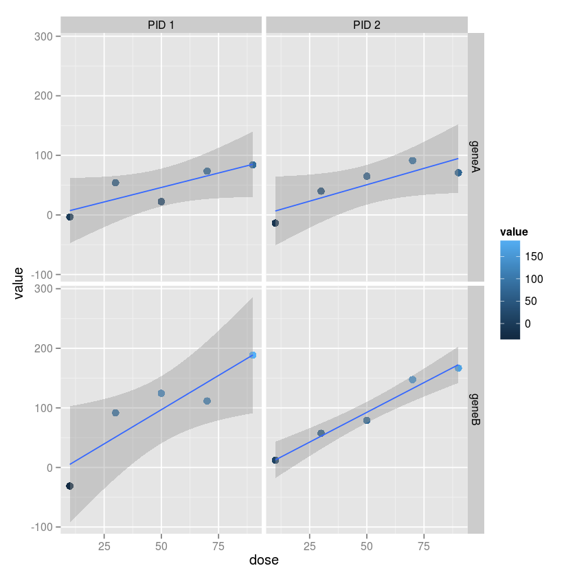
df <- data.frame(subject=subject, dose=dose, geneA=geneA, geneB=geneB)
df
| subject | dose | geneA | geneB | |
|---|---|---|---|---|
| 1 | PID 1 | 10 | -3.367338 | -31.18716 |
| 2 | PID 1 | 30 | 54.03613 | 91.78636 |
| 3 | PID 1 | 50 | 22.40099 | 124.477 |
| 4 | PID 1 | 70 | 73.61274 | 111.6039 |
| 5 | PID 1 | 90 | 84.05749 | 188.5058 |
| 6 | PID 2 | 10 | -13.63179 | 12.04911 |
| 7 | PID 2 | 30 | 40.03472 | 57.40407 |
| 8 | PID 2 | 50 | 64.98747 | 79.04738 |
| 9 | PID 2 | 70 | 91.22307 | 147.4357 |
| 10 | PID 2 | 90 | 70.94818 | 166.8696 |
Exercise 3
Using ggplot2, plot gene expression agaisnt does, using differnt
colors for differetn genes and differnet shapes for different subjects.
(Hint: The reshape2 library may come in useful)
md <- melt(df, id=c("subject", "dose"))
md
| subject | dose | variable | value | |
|---|---|---|---|---|
| 1 | PID 1 | 10 | geneA | -3.367338 |
| 2 | PID 1 | 30 | geneA | 54.03613 |
| 3 | PID 1 | 50 | geneA | 22.40099 |
| 4 | PID 1 | 70 | geneA | 73.61274 |
| 5 | PID 1 | 90 | geneA | 84.05749 |
| 6 | PID 2 | 10 | geneA | -13.63179 |
| 7 | PID 2 | 30 | geneA | 40.03472 |
| 8 | PID 2 | 50 | geneA | 64.98747 |
| 9 | PID 2 | 70 | geneA | 91.22307 |
| 10 | PID 2 | 90 | geneA | 70.94818 |
| 11 | PID 1 | 10 | geneB | -31.18716 |
| 12 | PID 1 | 30 | geneB | 91.78636 |
| 13 | PID 1 | 50 | geneB | 124.477 |
| 14 | PID 1 | 70 | geneB | 111.6039 |
| 15 | PID 1 | 90 | geneB | 188.5058 |
| 16 | PID 2 | 10 | geneB | 12.04911 |
| 17 | PID 2 | 30 | geneB | 57.40407 |
| 18 | PID 2 | 50 | geneB | 79.04738 |
| 19 | PID 2 | 70 | geneB | 147.4357 |
| 20 | PID 2 | 90 | geneB | 166.8696 |
ggplot(md, aes(x=dose, y=value, color=variable, shape=subject)) +
geom_point(size=5)
Exercise 4
Usign ggplot2, make a grid of plots with separae colummsn for each
subject and separate rows for each gene. Vary the color and size by the
gene expression value. Add a linear regression fit with 95% confidence
intervals to each plot.
ggplot(md, aes(x=dose, y=value, color=value)) +
geom_point(size=3) +
geom_smooth(method="lm") +
facet_grid(variable ~ subject)