Base Graphics¶

Building Graphs¶

Incremental building of features into graphs.

References

Graphical parameters
Colors
Named colors - type colors()
Using color scales and plattes in R
?plot
?par
Specific options e.g. ?pch

Basic plots¶

head(mtcars)

	mpg	cyl	disp	hp	drat	wt	qsec	vs	am	gear	carb
Mazda RX4	21	6	160	110	3.9	2.62	16.46	0	1	4	4
Mazda RX4 Wag	21	6	160	110	3.9	2.875	17.02	0	1	4	4
Datsun 710	22.8	4	108	93	3.85	2.32	18.61	1	1	4	1
Hornet 4 Drive	21.4	6	258	110	3.08	3.215	19.44	1	0	3	1
Hornet Sportabout	18.7	8	360	175	3.15	3.44	17.02	0	0	3	2
Valiant	18.1	6	225	105	2.76	3.46	20.22	1	0	3	1

with(mtcars, plot(wt, mpg))

scatter.smooth(mtcars$wt, mtcars$mpg)

df <- mtcars[order(mtcars$wt),]
with(df, plot(wt, mpg, type="b"))

with(mtcars, hist(mpg, breaks=10))

plot(density(mtcars$mpg), main="Density plot")

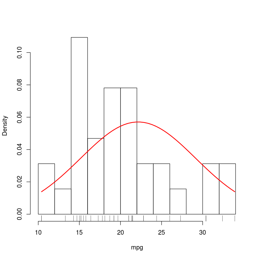
attach(mtcars)
hist(mpg, breaks=10, probability = TRUE, main="")
rug(mpg)
x <- seq(min(mpg), max(mpg), length.out = 50)
lines(x, dnorm(x, mean=mean(x), sd=sd(x)), col="red", lwd=2)
detach(mtcars)

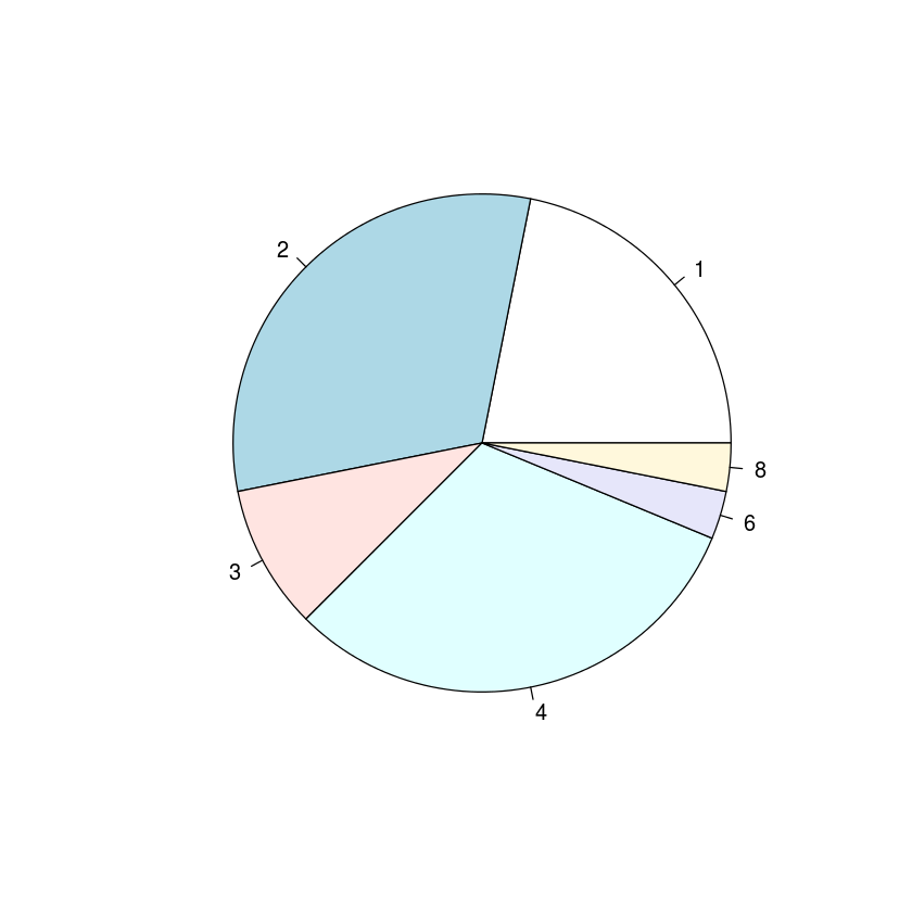
with(mtcars, pie(table(carb)))

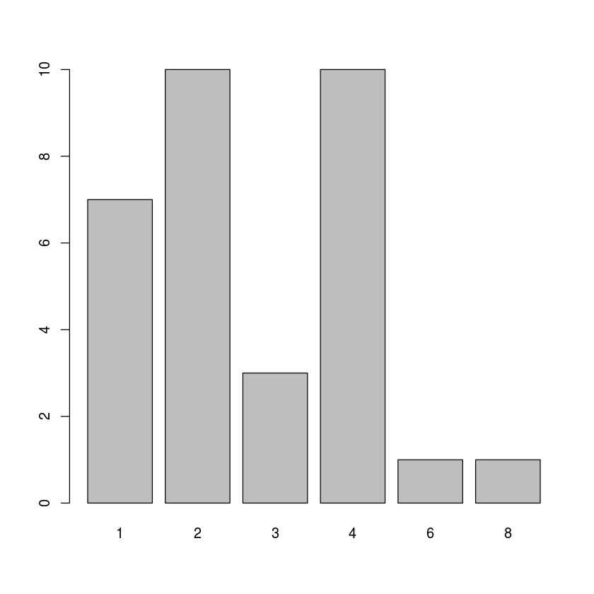
with(mtcars, barplot(table(carb)))

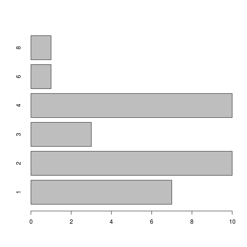
with(mtcars, barplot(table(carb), horiz=TRUE))

attach(mtcars)
(tbl <- table(carb, am))
barplot(tbl, beside=TRUE, legend=rownames(tbl), col=heat.colors(carb))
detach(mtcars)

BaseGraphics_files/BaseGraphics_16_0.png

boxplot(log1p(mtcars))

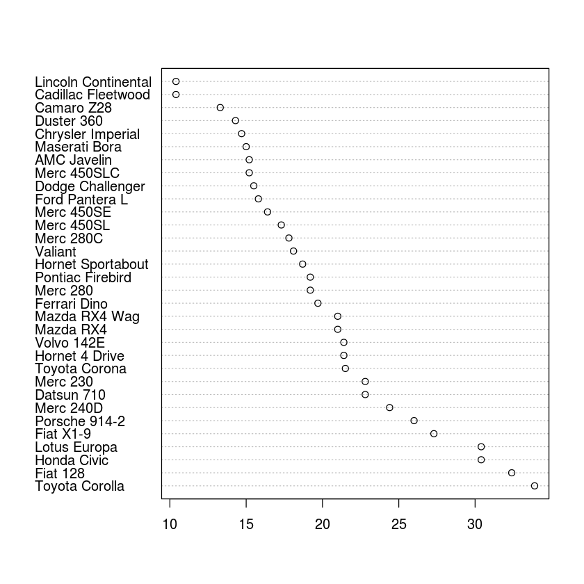
df <- mtcars[order(-mtcars$mpg),]
dotchart(df$mpg, labels=row.names(df))

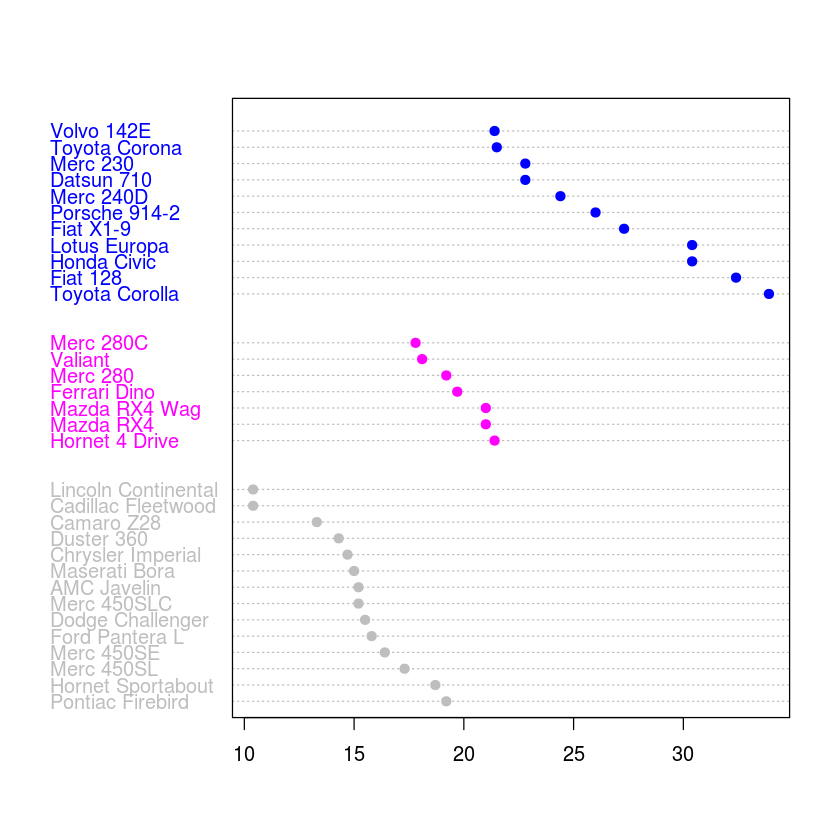
dotchart(df$mpg, labels=row.names(df), groups=df$cyl, color=df$cyl, pch=19)

pairs(~mpg + drat + wt, data=mtcars)

Building plots¶

Local customization of plots
Glaobl customization of plots
Adding more stuff to a plot
- points
- lines
- text
- mathematical expressions
Combining plots
Saving plots

Scatterplot¶

df <- mtcars[order(mtcars$wt),]
attach(df)
plot(wt, mpg)
detach(df)

Combining plots¶

par(mfrow=c(2,2))
plot(rnorm(10))
plot(rnorm(10))
plot(rnorm(10))
plot(rnorm(10))

(m <- matrix(c(1,1,2,3), 2, 2, byrow=TRUE))

1	1
2	3

layout(m)
plot(rnorm(10))
plot(rnorm(10))
plot(rnorm(10))

layout(m, widths=c(1,2), heights=c(2,1))
plot(rnorm(10))
plot(rnorm(10))
plot(rnorm(10))

orig <- par(no.readonly=TRUE)
x <- rnorm(10)
y <- rnorm(10)
par(fig = c(0, 0.8, 0, 0.8))
plot(x, y)
par(fig = c(0, 0.8, 0.6, 1), new=TRUE)
plot(density(x), axes=FALSE, main="", xlab="")
par(fig = c(0.6, 1, 0, 0.8), new=TRUE)
boxplot(y, axes=FALSE)
par(orig)

Plotting Graphcs and Heatmpas¶

Graphs¶

It may be necessary to install first

install.packages("igraphdata", repos = "http://cran.r-project.org")

library(igraph)
library(igraphdata)

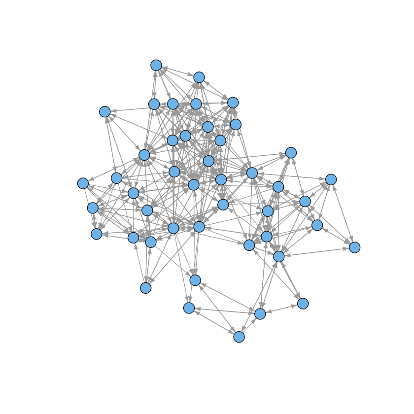
data(macaque)

plot(macaque, layout=layout.auto, vertex.shape="circle",
     vertex.size=8, edge.arrow.size=0.5, vertex.label=NA)

Heatmap¶

heatmap(as.matrix(mtcars), Rowv = NA, Colv = NA, scale = "column")

Heatmap with dendrogram¶

heatmap(as.matrix(mtcars), scale = "column")

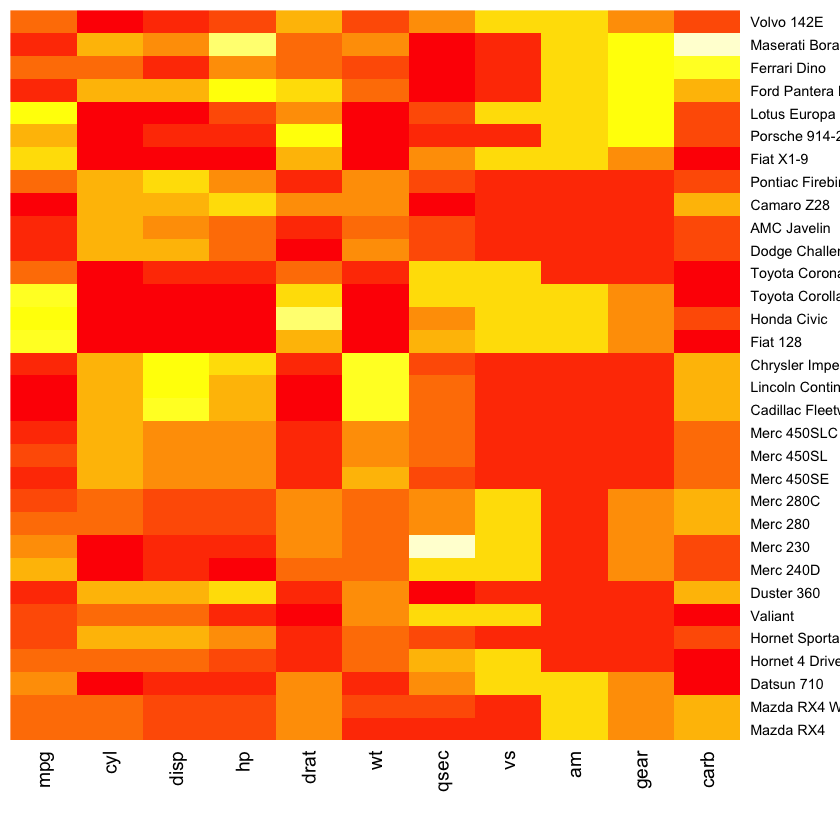
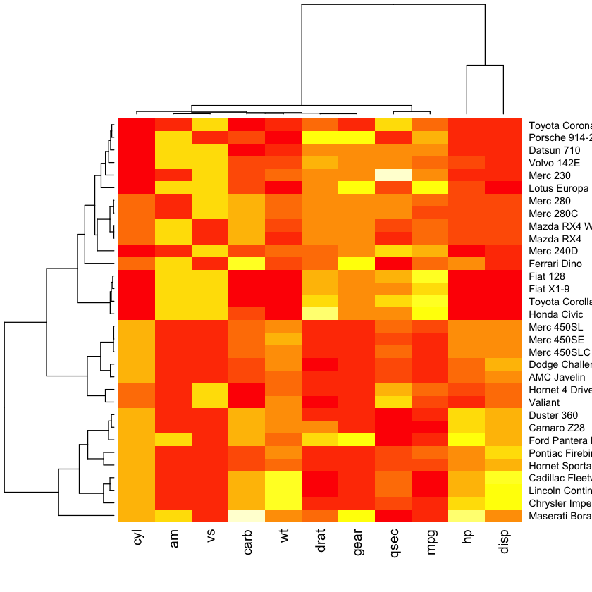
Fancy heatmaps¶

Also see d3heatmaps if you want an interactive heatmap. This does not seem to work within the notebook but will work in RStudio or an R script.

library(pheatmap)

pheatmap(as.matrix(mtcars), scale = "column")

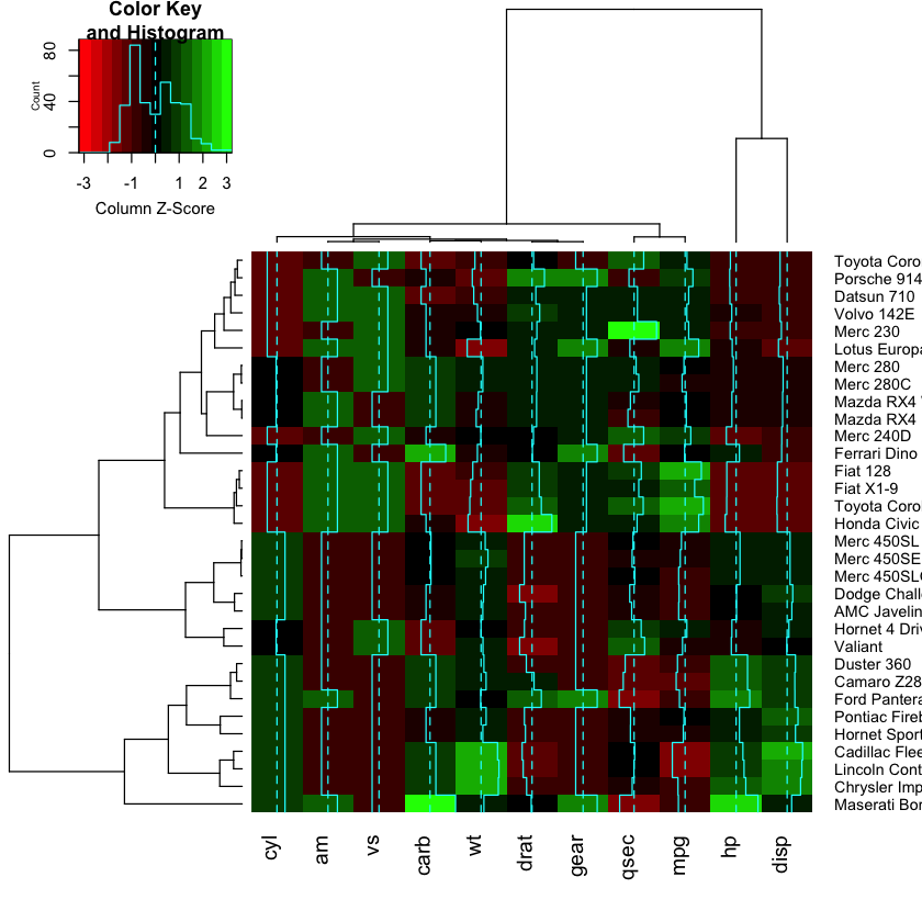
library(gplots)

heatmap.2(as.matrix(mtcars), scale = "column", col=redgreen)

Work!¶

Here we will try to replicate the noise discovery heatmap shown in the statistics class.

suppressMessages(library(genefilter))

Perform noise discovery¶

set.seed(123)

n <- 20 # number of subjects
m <- 20000 # number of genes
alpha <- 0.005 # significance level

# create a matrix of gene expression values with m rows and 2*n columns
M <- matrix(rnorm(2*n*m), m, 2*n)

# give row and column names
rownames(M) <- paste("G", 1:m, sep="")
colnames(M) <- paste("id", 1:(2*n), sep="")

# assign subjects inot equal sized groups
grp <- factor(rep(0:1, c(n, n)))

# calculate p-value using t-test for mean experession value of each gene
pvals <- rowttests(M, grp)$p.value

# extract the genes which meet the specified significance level
hits <- M[pvals < alpha,]

Use pheatmap to plot a heatmap
Remove the row names (Google or use R’s built-in help to figure out to do this)
Use this color palette to map expression values to a red-blakc-green scale

colorRampPalette(c("red3", "black", "green3"))(50)