Introduction to R¶

Loading libraries¶

Some R functions are in libraries that have to be explicitly loaded. You do this with the library command. The next cell shows an example of loading the genefilter library which contains the rowttests fucntion that we will be using later.

library(genefilter)

Attaching package: ‘genefilter’

The following object is masked from ‘package:base’:

    anyNA

Installing libraries¶

Most libraries have been pre-installed on the VM. However, if you need to install a new library, all you need is to use the install.packages() function. For example, you can install the MASS (Modern Applied Statistics in S) library like so:

install.packages("MASS", repos = "http://cran.r-project.org")

Some specialized libraries come from the R BioConductor project, and the installation processs is slgihtly different. This will be covered in a later session.

R as simple calculator¶

2 + 3^5

7 %% 3

sin(0.5*pi)

1.23e3

Printing results¶

By default, the result on the last line is displayed in the Jupyter notebook. To see other lines, use the print function.

print(1 * 2 * 3 *4)
print(11 %% 3 == 1)
10 > 1

[1] 24
[1] FALSE

Getting help¶

Type soemthing and hit the tab key - this will either complete the R command for you (if unique) or present a list of opitons.

Use ?topic to get a description of topic, or more verbosely, you can also use help(topic).

?seq

Sequence Generation

Description

Generate regular sequences. seq is a standard generic with a default method. seq.int is a primitive which can be much faster but has a few restrictions. seq_along and seq_len are very fast primitives for two common cases.

Usage

seq(...)

## Default S3 method:
seq(from = 1, to = 1, by = ((to - from)/(length.out - 1)),
    length.out = NULL, along.with = NULL, ...)

seq.int(from, to, by, length.out, along.with, ...)

seq_along(along.with)
seq_len(length.out)

Arguments

Details

Numerical inputs should all be finite (that is, not infinite, NaN or NA).

The interpretation of the unnamed arguments of seq and seq.int is not standard, and it is recommended always to name the arguments when programming.

seq is generic, and only the default method is described here. Note that it dispatches on the class of the first argument irrespective of argument names. This can have unintended consequences if it is called with just one argument intending this to be taken as along.with: it is much better to use seg_along in that case.

seq.int is an internal generic which dispatches on methods for "seq" based on the class of the first supplied argument (before argument matching).

Typical usages are

seq(from, to)
seq(from, to, by= )
seq(from, to, length.out= )
seq(along.with= )
seq(from)
seq(length.out= )

The first form generates the sequence from, from+/-1, ..., to (identical to from:to).

The second form generates from, from+by, ..., up to the sequence value less than or equal to to. Specifying to - from and by of opposite signs is an error. Note that the computed final value can go just beyond to to allow for rounding error, but is truncated to to. (‘Just beyond’ is by up to 1e-10 times abs(from - to).)

The third generates a sequence of length.out equally spaced values from from to to. (length.out is usually abbreviated to length or len, and seq_len is much faster.)

The fourth form generates the integer sequence 1, 2, ..., length(along.with). (along.with is usually abbreviated to along, and seq_along is much faster.)

The fifth form generates the sequence 1, 2, ..., length(from) (as if argument along.with had been specified), unless the argument is numeric of length 1 when it is interpreted as 1:from (even for seq(0) for compatibility with S). Using either seq_along or seq_len is much preferred (unless strict S compatibility is essential).

The final form generates the integer sequence 1, 2, ..., length.out unless length.out = 0, when it generates integer(0).

Very small sequences (with from - to of the order of 10^{-14} times the larger of the ends) will return from.

For seq (only), up to two of from, to and by can be supplied as complex values provided length.out or along.with is specified. More generally, the default method of seq will handle classed objects with methods for the Math, Ops and Summary group generics.

seq.int, seq_along and seq_len are primitive.

Value

seq.int and the default method of seq for numeric arguments return a vector of type "integer" or "double": programmers should not rely on which.

seq_along and seq_len return an integer vector, unless it is a long vector when it will be double.

References

Becker, R. A., Chambers, J. M. and Wilks, A. R. (1988) The New S Language. Wadsworth & Brooks/Cole.

See Also

The methods seq.Date and seq.POSIXt.

:, rep, sequence, row, col.

Examples

seq(0, 1, length.out = 11)
seq(stats::rnorm(20)) # effectively 'along'
seq(1, 9, by = 2)     # matches 'end'
seq(1, 9, by = pi)    # stays below 'end'
seq(1, 6, by = 3)
seq(1.575, 5.125, by = 0.05)
seq(17) # same as 1:17, or even better seq_len(17)

Use example to see usage examples.

example(seq)

seq> seq(0, 1, length.out = 11)
 [1] 0.0 0.1 0.2 0.3 0.4 0.5 0.6 0.7 0.8 0.9 1.0

seq> seq(stats::rnorm(20)) # effectively 'along'
 [1]  1  2  3  4  5  6  7  8  9 10 11 12 13 14 15 16 17 18 19 20

seq> seq(1, 9, by = 2)     # matches 'end'
[1] 1 3 5 7 9

seq> seq(1, 9, by = pi)    # stays below 'end'
[1] 1.000000 4.141593 7.283185

seq> seq(1, 6, by = 3)
[1] 1 4

seq> seq(1.575, 5.125, by = 0.05)
 [1] 1.575 1.625 1.675 1.725 1.775 1.825 1.875 1.925 1.975 2.025 2.075 2.125
[13] 2.175 2.225 2.275 2.325 2.375 2.425 2.475 2.525 2.575 2.625 2.675 2.725
[25] 2.775 2.825 2.875 2.925 2.975 3.025 3.075 3.125 3.175 3.225 3.275 3.325
[37] 3.375 3.425 3.475 3.525 3.575 3.625 3.675 3.725 3.775 3.825 3.875 3.925
[49] 3.975 4.025 4.075 4.125 4.175 4.225 4.275 4.325 4.375 4.425 4.475 4.525
[61] 4.575 4.625 4.675 4.725 4.775 4.825 4.875 4.925 4.975 5.025 5.075 5.125

seq> seq(17) # same as 1:17, or even better seq_len(17)
 [1]  1  2  3  4  5  6  7  8  9 10 11 12 13 14 15 16 17

To search for all functions with the phrase topic, use apropos(topic).

apropos("seq")

1. 'seq'
2. 'seq_along'
3. 'seq.Date'
4. 'seq.default'
5. 'seq.int'
6. 'seq_len'
7. 'seq.POSIXt'
8. 'sequence'

For a broader search using “fuzzy” matching, use ?? prepended to the search term.

??seq

Finally, you can always use a search engine - e.g. Googling for “how to generate random numbers from a normal distribution in R” returens:

R Learning Module: Probabilities and Distributions www.ats.ucla.edu › stat › r › modules University of California, Los Angeles Generating random samples from a normal distribution ... (For more information on the random number generator used in R please refer to the help pages for the ...

R: The Normal Distribution https://stat.ethz.ch/R-manual/R-devel/library/.../Normal.html ETH Zurich Normal {stats}, R Documentation ... quantile function and random generation for the normal distribution with mean equal to mean and ... number of observations.

CASt R: Random numbers astrostatistics.psu.edu/.../R/Random.html Pennsylvania State University It is often necessary to simulate random numbers in R. There are many functions available to ... Let’s consider the well-known normal distribution as an example: ?Normal .... Creating functions in R, as illustrated above, is a common procedure.

Assigning to variables¶

x <- 3
y <- 5

z <- x * y

z

Creating and using sequences¶

1:4

1. 1
2. 2
3. 3
4. 4

seq(2, 12, 3)

1. 2
2. 5
3. 8
4. 11

seq(from=0, to=pi, by=pi/4)

1. 0
2. 0.785398163397448
3. 1.5707963267949
4. 2.35619449019234
5. 3.14159265358979

seq(from=0, to=pi, length.out = 5)

1. 0
2. 0.785398163397448
3. 1.5707963267949
4. 2.35619449019234
5. 3.14159265358979

Vectorized operations¶

x <- 1:10
y <- 1:10

x * y

1. 1
2. 4
3. 9
4. 16
5. 25
6. 36
7. 49
8. 64
9. 81
10. 100

x <- seq(0, 2*pi, length.out = 5)
sin(x)

1. 0
2. 1
3. 1.22464679914735e-16
4. -1
5. -2.44929359829471e-16

Functions¶

A function is code tha behaves like a black box - you give it some input and it returns some output. Functions are essenital because they allow you to design use potentially complicated algorithms without having to keep track of the algorithmic details - all you need to remeber are the function name (which you can search with apropos or prepnding ?? to the search term), the input arguments (TAB provides hings), and what type of output will be generated. Most of R’s usefulness comes from the large collection of functions that it provides - for example, library(), seq(), as.fractions() are all functions. You can also write your own R functions - this will be covered in detail in a later session - but we show the basics here so that you can follow the statistics lecutures.

A function has the following structure

function_name <- function(arguments) {
    body_of_function
    return(result)
    }

The simple example below will make this explicit.

my.func <- function(a, b) {
    c <- a * b
    return(a + b - c)
    }

my.func(5, 4)

my.func(b=4, a=5)

sum.odd(1, 100)

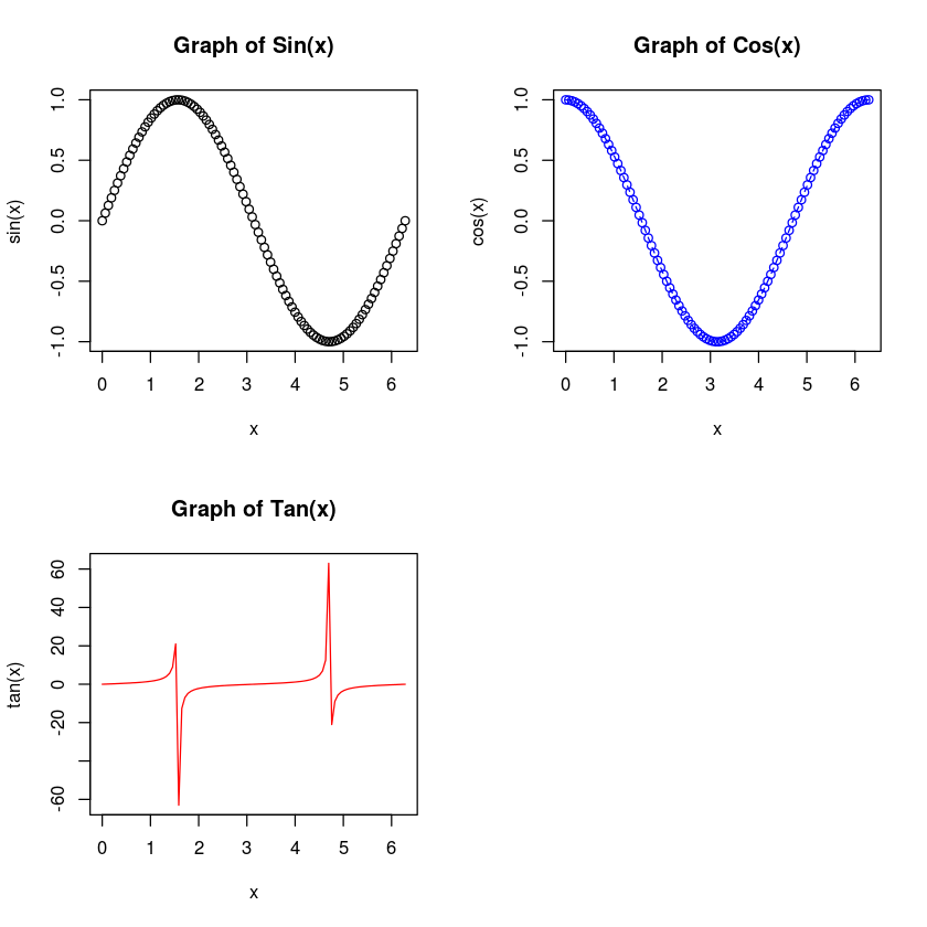
Graphics¶

x <- seq(0, 2*pi, length.out = 100)
plot(x, sin(x), main="Graph of Sin(x)")

par(mfrow=c(2,2))
plot(x, sin(x), main="Graph of Sin(x)")
plot(x, cos(x), main="Graph of Cos(x)", type="o", col="blue", lty=2)
plot(x, tan(x), main="Graph of Tan(x)", type="l", col="red")

The concept of “saving” a graphical plot in R involves the following steps

• open a “device” to plot to (the next shows a pdf device)
  • this includes the filename and other configuration parameters such as width and height
• write all the plotting and customization commands as usual
• close the device with dev.close() - this writes the plot to file

pdf("trig.pdf", width=12, height=4)
par(mfrow=c(1,3))
plot(x, sin(x), main="Graph of Sin(x)")
plot(x, cos(x), main="Graph of Cos(x)", type="o", col="blue", lty=2)
plot(x, tan(x), main="Graph of Tan(x)", type="l", col="red")
dev.off()

?device

List of Graphical Devices

Description

The following graphics devices are currently available:

• pdf Write PDF graphics commands to a file

• postscript Writes PostScript graphics commands to a file

• xfig Device for XFIG graphics file format

• bitmap bitmap pseudo-device via Ghostscript (if available).

• pictex Writes TeX/PicTeX graphics commands to a file (of historical interest only)

The following devices will be functional if R was compiled to use them (they exist but will return with a warning on other systems):

• X11 The graphics device for the X11 windowing system

• cairo_pdf, cairo_ps PDF and PostScript devices based on cairo graphics.

• svg SVG device based on cairo graphics.

• png PNG bitmap device

• jpeg JPEG bitmap device

• bmp BMP bitmap device

• tiff TIFF bitmap device

• quartz The graphics device for the OS X native Quartz 2d graphics system. (This is only functional on OS X where it can be used from the R.app GUI and from the command line: but it will display on the local screen even for a remote session.)

Details

If no device is open, using a high-level graphics function will cause a device to be opened. Which device is given by options("device") which is initially set as the most appropriate for each platform: a screen device for most interactive use and pdf (or the setting of R_DEFAULT_DEVICE) otherwise. The exception is interactive use under Unix if no screen device is known to be available, when pdf() is used.

It is possible for an R package to provide further graphics devices and several packages on CRAN do so. These include other devices outputting SVG and PGF/TiKZ (TeX-based graphics, see http://pgf.sourceforge.net/).

See Also

The individual help files for further information on any of the devices listed here; X11.options, quartz.options, ps.options and pdf.options for how to customize devices.

dev.interactive, dev.cur, dev.print, graphics.off, image, dev2bitmap.

capabilities to see if X11, jpeg png, tiff, quartz and the cairo-based devices are available.

Examples

## Not run:
## open the default screen device on this platform if no device is
## open
if(dev.cur() == 1) dev.new()

## End(Not run)

Introudction to simulations¶

The statistics lectures will use statistical simulations extensively to illustrate key concepts. Basically, a simulaition is the use of random numbers drawn from some probability distribution to simulate experimental results. Simulations are a wonderful way to learn more about probability distributions and the concepts behind statistical inference.

set.seed(123) # fix random number seed for reproducibility

(x <- c("H", "T"))

1. 'H'
2. 'T'

sample(x, 20, replace=TRUE)

1. 'T'
2. 'H'
3. 'H'
4. 'T'
5. 'T'
6. 'H'
7. 'T'
8. 'T'
9. 'H'
10. 'T'
11. 'T'
12. 'T'
13. 'H'
14. 'H'
15. 'H'
16. 'T'
17. 'T'
18. 'H'
19. 'T'
20. 'H'

(x <- 1:6)

1. 1
2. 2
3. 3
4. 4
5. 5
6. 6

sample(x, 10, replace=FALSE)

Error in sample.int(length(x), size, replace, prob): cannot take a sample larger than the population when 'replace = FALSE'

sample(x)

1. 1
2. 6
3. 4
4. 3
5. 2
6. 5

sample(x)

1. 3
2. 4
3. 2
4. 1
5. 6
6. 5

sample(x, size = 3)

1. 3
2. 2
3. 5

sample(x, size=10, replace=TRUE, prob=c(10,10,10,1,1,1))

1. 3
2. 3
3. 4
4. 1
5. 2
6. 1
7. 1
8. 3
9. 1
10. 3

Continuous distributions¶

par(mfrow=c(2,2)) # arrange plots in a 2 x 2 grid

x <- rnorm(n=100, mean=0, sd=1)
hist(x, main="Normal distribution")
rug(x)

x <- rexp(n=100, rate = 1)
hist(x, main="Exponenital distribution")
rug(x)

x <- runif(n=100, min=0, max=10)
hist(x, main="Uniform distribution")
rug(x)

x <- rbeta(n=100, shape1 = 0.5, shape2=0.5)
hist(x, main="Beta distribution")
rug(x)

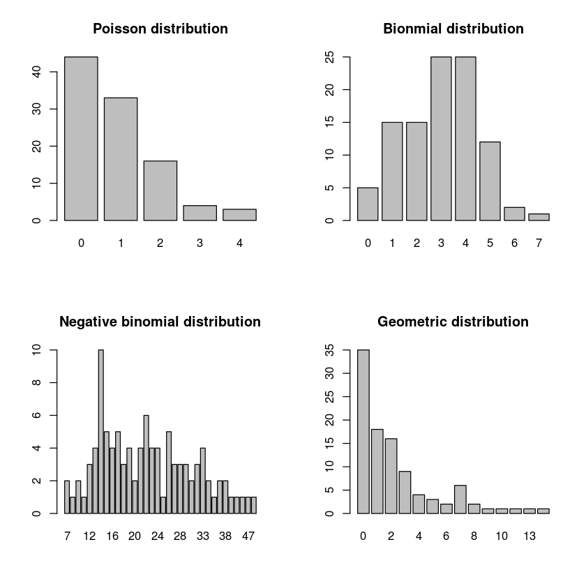
Discrete distributions¶

par(mfrow=c(2,2)) # arrange plots in a 2 x 2 grid

x <- rpois(n=100, lambda = 1)
barplot(table(x), main="Poisson distribution")

x <- rbinom(n=100, size=10, prob=0.3)
barplot(table(x), main="Bionmial distribution")

x <- rnbinom(n=100, size=10, prob=0.3)
barplot(table(x), main="Negative binomial distribution")

x <- rgeom(n=100, prob=0.3)
barplot(table(x), main="Geometric distribution")

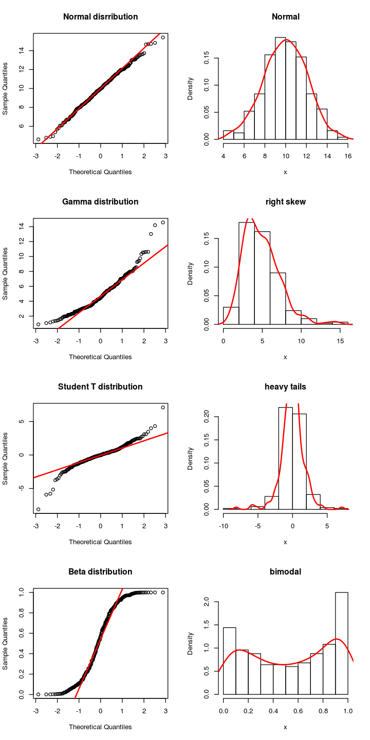
Checking distributions with qqplot¶

Most commonly, we want to check if data comes from a normal distribution. To do this, we can plot the sample quantiles against the theoretical quantiles - if the data is normally distributed, this should not deviate far from a straight line. To chack against a normal distribution, use qqnorm(x) where x is the sample to be tested. More generally, you can test if x comes from any distribution using qqplot(x, dist).

options(repr.plot.width = 6)
options(repr.plot.height = 12)
par(mfrow=c(4,2))

n <- 250

x <- rnorm(n=n, mean=10, sd=2)
qqnorm(x, main="Normal disrribution")
qqline(x, col="red", lwd=2)

hist(x, probability = TRUE, main="Normal")
lines(density(x), col="red", lwd=2)

x <- rgamma(n=n, scale=1, shape=5)
qqnorm(x, main="Gamma distribution")
qqline(x, col="red", lwd=2)

hist(x, probability = TRUE, main="right skew")
lines(density(x), col="red", lwd=2)

x <- rt(n=n, df=3)
qqnorm(x, main="Student T distribution")
qqline(x, col="red", lwd=2)

hist(x, probability = TRUE, main="heavy tails")
lines(density(x), col="red", lwd=2)

x <- rbeta(n=n, shape1 = 0.5, shape2=0.5)
qqnorm(x, main="Beta distribution")
qqline(x, col="red", lwd=2)

hist(x, probability = TRUE, main="bimodal")
lines(density(x), col="red", lwd=2)

A simple simulation¶

How frequently do we find significant differences (p < 0.05) between two groups when they are drawn from the same distribuiton if we use a t test?

As a bonus, this code snippet also shows a simple way to time chunks of code.

Digression - using Loops¶

To repeat an action many times, we use loops. The most useful loop construct in R is the for loop. A simple example shows how to use it.

for (i in 1:4) {
    print(c(i, i*i))
    }

[1] 1 1
[1] 2 4
[1] 3 9
[1]  4 16

Loops many include an if condition to only run the code if some condition is met.

for (i in 1:4) {
    if (i %% 2 == 0) { # is i an even number?
        print(c(i, i*i))
        }
    }

[1] 2 4
[1]  4 16

Now that we know how to use loops, let’s write the actural simulation.

nexpts = 10000
nsamps = 100
s = 0
alpha = 0.05

ptm <- proc.time()
for (i in 1:nexpts) {
    u <- rnorm(nsamps)
    v <- rnorm(nsamps)
    if (t.test(u, v)$p.value < alpha)
        s = s + 1
}
print(s/nexpts)

proc.time() - ptm

[1] 0.047

 user  system elapsed
2.544   0.006   2.551

ptm <- proc.time()
x <- matrix(rnorm(2*nexpts*nsamps), nexpts, 2*nsamps)
grp <- factor(rep(0:1, c(nsamps, nsamps)))
print(sum(rowttests(x, grp)$p.value < alpha)/nexpts)

proc.time() - ptm

[1] 0.0507

 user  system elapsed
0.544   0.017   0.562