Practice 2
Working with dataframes
Practice TWO is meant to help you get comfortable working with data frames, and the basic ways you can slice and dice datafrmaes.
- How many rows and columns are there in the
mtcarsdataframe?
(nrow(mtcars))
(ncol(mtcars))
[1] 32
[1] 11
dim(mtcars)
[1] 32 11
- Show the last 6 rows of
mtcars.
tail(mtcars, 6)
                mpg cyl  disp  hp drat    wt qsec vs am gear carb
Porsche 914-2  26.0   4 120.3  91 4.43 2.140 16.7  0  1    5    2
Lotus Europa   30.4   4  95.1 113 3.77 1.513 16.9  1  1    5    2
Ford Pantera L 15.8   8 351.0 264 4.22 3.170 14.5  0  1    5    4
Ferrari Dino   19.7   6 145.0 175 3.62 2.770 15.5  0  1    5    6
Maserati Bora  15.0   8 301.0 335 3.54 3.570 14.6  0  1    5    8
Volvo 142E     21.4   4 121.0 109 4.11 2.780 18.6  1  1    4    2
- Show 6 rows at random (no duplicates) from
mtcars
ridx <- sample(1:nrow(mtcars), 6, replace=FALSE)
mtcars[ridx,]
               mpg cyl  disp  hp drat    wt  qsec vs am gear carb
Toyota Corona 21.5   4 120.1  97 3.70 2.465 20.01  1  0    3    1
Camaro Z28    13.3   8 350.0 245 3.73 3.840 15.41  0  0    3    4
Valiant       18.1   6 225.0 105 2.76 3.460 20.22  1  0    3    1
Merc 280C     17.8   6 167.6 123 3.92 3.440 18.90  1  0    4    4
Fiat 128      32.4   4  78.7  66 4.08 2.200 19.47  1  1    4    1
AMC Javelin   15.2   8 304.0 150 3.15 3.435 17.30  0  0    3    2
- Display information only for the subset of cars with automatic transmission.
mtcars[mtcars$am == 1,]
                mpg cyl  disp  hp drat    wt  qsec vs am gear carb
Mazda RX4      21.0   6 160.0 110 3.90 2.620 16.46  0  1    4    4
Mazda RX4 Wag  21.0   6 160.0 110 3.90 2.875 17.02  0  1    4    4
Datsun 710     22.8   4 108.0  93 3.85 2.320 18.61  1  1    4    1
Fiat 128       32.4   4  78.7  66 4.08 2.200 19.47  1  1    4    1
Honda Civic    30.4   4  75.7  52 4.93 1.615 18.52  1  1    4    2
Toyota Corolla 33.9   4  71.1  65 4.22 1.835 19.90  1  1    4    1
Fiat X1-9      27.3   4  79.0  66 4.08 1.935 18.90  1  1    4    1
Porsche 914-2  26.0   4 120.3  91 4.43 2.140 16.70  0  1    5    2
Lotus Europa   30.4   4  95.1 113 3.77 1.513 16.90  1  1    5    2
Ford Pantera L 15.8   8 351.0 264 4.22 3.170 14.50  0  1    5    4
Ferrari Dino   19.7   6 145.0 175 3.62 2.770 15.50  0  1    5    6
Maserati Bora  15.0   8 301.0 335 3.54 3.570 14.60  0  1    5    8
Volvo 142E     21.4   4 121.0 109 4.11 2.780 18.60  1  1    4    2
- Display information only for the subset of cars with weight between 2 and 3.
mtcars[(2 < mtcars$wt) & (mtcars$wt < 3),]
               mpg cyl  disp  hp drat    wt  qsec vs am gear carb
Mazda RX4     21.0   6 160.0 110 3.90 2.620 16.46  0  1    4    4
Mazda RX4 Wag 21.0   6 160.0 110 3.90 2.875 17.02  0  1    4    4
Datsun 710    22.8   4 108.0  93 3.85 2.320 18.61  1  1    4    1
Fiat 128      32.4   4  78.7  66 4.08 2.200 19.47  1  1    4    1
Toyota Corona 21.5   4 120.1  97 3.70 2.465 20.01  1  0    3    1
Porsche 914-2 26.0   4 120.3  91 4.43 2.140 16.70  0  1    5    2
Ferrari Dino  19.7   6 145.0 175 3.62 2.770 15.50  0  1    5    6
Volvo 142E    21.4   4 121.0 109 4.11 2.780 18.60  1  1    4    2
- What is the mean weight of all cars?
mean(mtcars$wt)
[1] 3.21725
(7) What is the mean weight of cars wtih `mpg` greater than 20?
mean(mtcars[mtcars$mpg > 20, "wt"])
[1] 2.418071
- Add a column
kplshowing the number of kilometers per liter (1 mile = 1.609344 kilometers, and 1 gallon = 3.78541178 liters)
mpg.to.kpl <- function(mpg) {
    return(mpg * 1.609344 / 3.78541178)
}
mtcars$kpl <- mpg.to.kpl(mtcars$mpg)
head(mtcars)
                   mpg cyl disp  hp drat    wt  qsec vs am gear carb      kpl
Mazda RX4         21.0   6  160 110 3.90 2.620 16.46  0  1    4    4 8.928018
Mazda RX4 Wag     21.0   6  160 110 3.90 2.875 17.02  0  1    4    4 8.928018
Datsun 710        22.8   4  108  93 3.85 2.320 18.61  1  1    4    1 9.693277
Hornet 4 Drive    21.4   6  258 110 3.08 3.215 19.44  1  0    3    1 9.098075
Hornet Sportabout 18.7   8  360 175 3.15 3.440 17.02  0  0    3    2 7.950187
Valiant           18.1   6  225 105 2.76 3.460 20.22  1  0    3    1 7.695101
- Make a new dataframe
mtcars.1with only thempgandkplcolumns.
mtcars.1 <- mtcars[, c("mpg", "kpl")]
head(mtcars.1)
                   mpg      kpl
Mazda RX4         21.0 8.928018
Mazda RX4 Wag     21.0 8.928018
Datsun 710        22.8 9.693277
Hornet 4 Drive    21.4 9.098075
Hornet Sportabout 18.7 7.950187
Valiant           18.1 7.695101
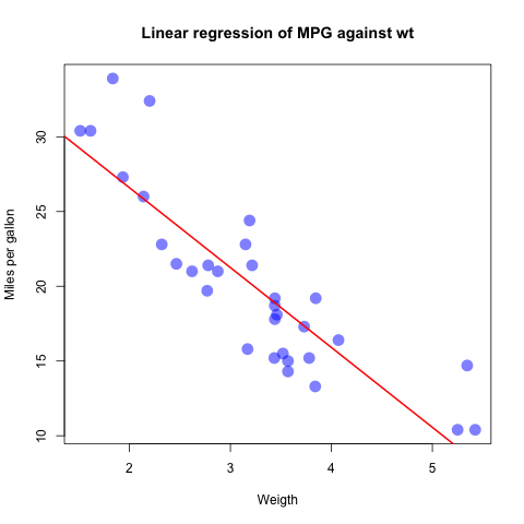
- Perform a linear regression model of
mpgagainstwt. Plot the model fit.
fit <- lm(mpg ~ wt, data=mtcars)
summary(fit)
Call:
lm(formula = mpg ~ wt, data = mtcars)

Residuals:
    Min      1Q  Median      3Q     Max
-4.5432 -2.3647 -0.1252  1.4096  6.8727

Coefficients:
            Estimate Std. Error t value Pr(>|t|)
(Intercept)  37.2851     1.8776  19.858  < 2e-16 *
wt           -5.3445     0.5591  -9.559 1.29e-10 *
---
Signif. codes:  0 ‘*’ 0.001 ‘’ 0.01 ‘*’ 0.05 ‘.’ 0.1 ‘ ’ 1

Residual standard error: 3.046 on 30 degrees of freedom
Multiple R-squared:  0.7528,        Adjusted R-squared:  0.7446
F-statistic: 91.38 on 1 and 30 DF,  p-value: 1.294e-10
plot(mtcars$wt, mtcars$mpg, col=rgb(0,0,1,0.5), pch=16, cex=2.0,
    xlab="Weigth", ylab="Miles per gallon",
     main="Linear regression of MPG against wt")
abline(fit, col="red", lwd=2)
- Print 10 rows at ranodm from the
irisdataframe
ridx <- sample(1:nrow(iris), 10, replace = FALSE)
iris[ridx,]
    Sepal.Length Sepal.Width Petal.Length Petal.Width    Species
136          7.7         3.0          6.1         2.3  virginica
10           4.9         3.1          1.5         0.1     setosa
29           5.2         3.4          1.4         0.2     setosa
80           5.7         2.6          3.5         1.0 versicolor
54           5.5         2.3          4.0         1.3 versicolor
11           5.4         3.7          1.5         0.2     setosa
58           4.9         2.4          3.3         1.0 versicolor
56           5.7         2.8          4.5         1.3 versicolor
150          5.9         3.0          5.1         1.8  virginica
59           6.6         2.9          4.6         1.3 versicolor
- Find the mean Sepal.Length Sepal.Width Petal.Length Petal.Width for
each iris species using the
aggregatecommand.
aggregate(iris[,1:4], by=list(iris$Species), FUN=mean)
     Group.1 Sepal.Length Sepal.Width Petal.Length Petal.Width
1     setosa        5.006       3.428        1.462       0.246
2 versicolor        5.936       2.770        4.260       1.326
3  virginica        6.588       2.974        5.552       2.026