More `ggplot2`¶

Using `ggplot2` (Grammar of Graphics)¶

In addition to the base plotting facilites we have been using, R also has the ggplot2 package that can be used to generate beutfiul graphs. We will only touch on a small subset of ggplot2 capabiliites here.

References

R Graphics Cookbook

library(ggplot2)
library(grid)
library(gridExtra)

head(mtcars)

	mpg	cyl	disp	hp	drat	wt	qsec	vs	am	gear	carb
Mazda RX4	21	6	160	110	3.9	2.62	16.46	0	1	4	4
Mazda RX4 Wag	21	6	160	110	3.9	2.875	17.02	0	1	4	4
Datsun 710	22.8	4	108	93	3.85	2.32	18.61	1	1	4	1
Hornet 4 Drive	21.4	6	258	110	3.08	3.215	19.44	1	0	3	1
Hornet Sportabout	18.7	8	360	175	3.15	3.44	17.02	0	0	3	2
Valiant	18.1	6	225	105	2.76	3.46	20.22	1	0	3	1

Chaining plotting functions¶

ggplot()
aes()
geom_xxx()
annotationa

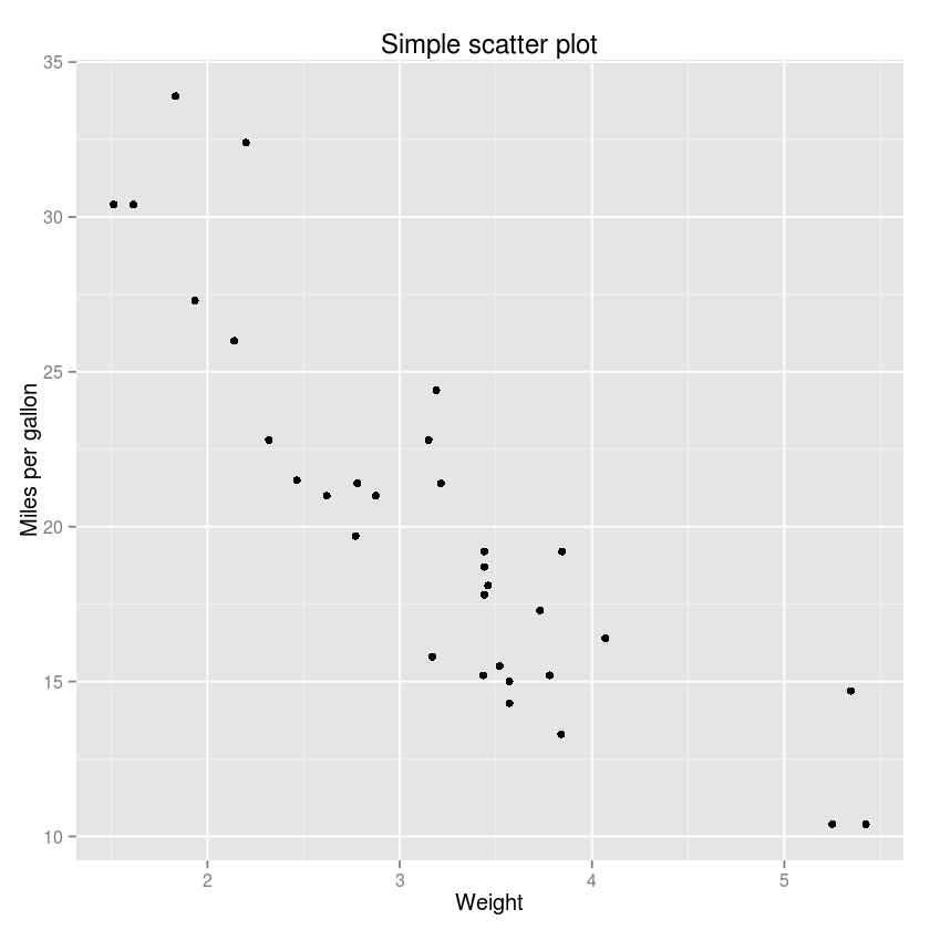
ggplot(data=mtcars, aes(x=wt, y=mpg)) +
geom_point() +
labs(title="Simple scatter plot", x="Weight", y="Miles per gallon")

_images/GGPlot2Graphics_5_0.png

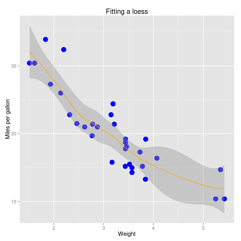
ggplot(data=mtcars, aes(x=wt, y=mpg)) +
geom_point(color="blue", size=5) +
geom_smooth(method="loess", color="orange") +
labs(title="Fitting a loess", x="Weight", y="Miles per gallon")

_images/GGPlot2Graphics_6_0.png

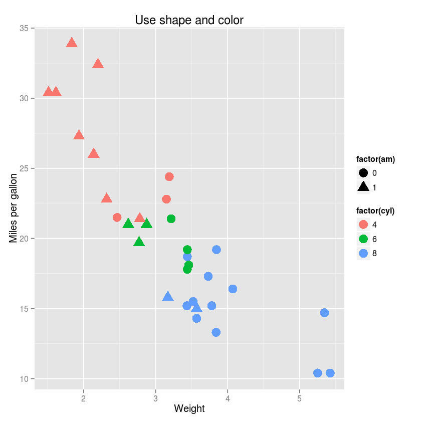
ggplot(data=mtcars, aes(x=wt, y=mpg, color=factor(cyl),, shape=factor(am))) +
geom_point(size=5) +
labs(title="Use shape and color", x="Weight", y="Miles per gallon")

_images/GGPlot2Graphics_7_0.png

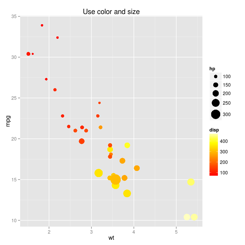
p <- ggplot(mtcars, aes(x=wt, y=mpg))
p +
geom_point(aes(size=hp, color=disp)) +
ggtitle("Use color and size") +
scale_colour_gradientn(colours=heat.colors(10)) +
scale_size(range=c(2, 10))

_images/GGPlot2Graphics_8_0.png

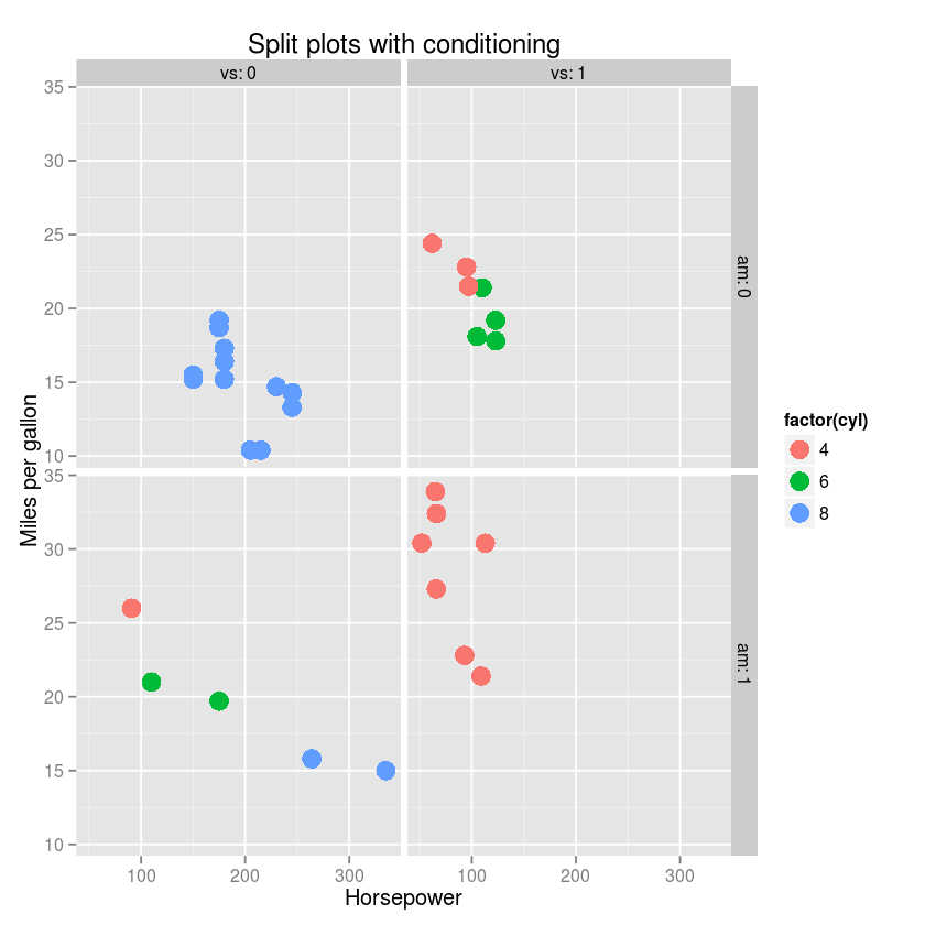
ggplot(data=mtcars, aes(x=hp, y=mpg, color=factor(cyl))) +
geom_point(size=5) +
facet_grid(am ~ vs, labeller = label_both) +
labs(title="Split plots with conditioning", x="Horsepower", y="Miles per gallon")

_images/GGPlot2Graphics_9_0.png

More examples¶

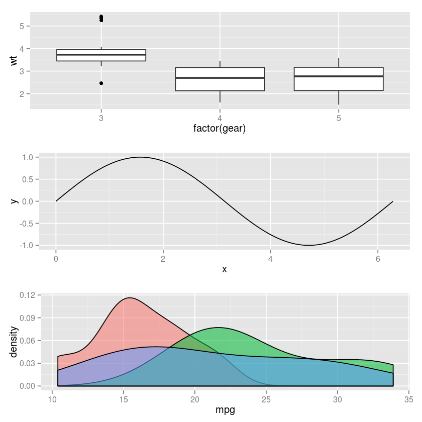
p4 <- ggplot(mtcars, aes(x=factor(gear), y=wt)) +
      geom_boxplot()
p5 <- ggplot(data.frame(x=seq(0, 2*pi, length.out = 50)), aes(x=x)) +
      stat_function(fun=sin, geom="line")
p6 <- ggplot(mtcars, aes(x=mpg, alpha=0.5, fill=factor(gear))) +
      geom_density() +
      guides(alpha=FALSE, fill=FALSE)
grid.arrange(p4, p5, p6, ncol = 1)

_images/GGPlot2Graphics_11_0.png

Plot aesthetics¶

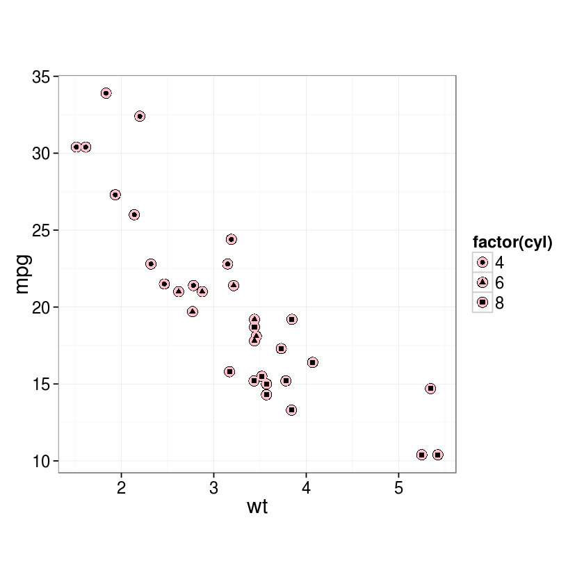
ggplot(mtcars, aes(x=wt, y=mpg)) +
geom_point(colour="black", size = 4.5, show_guide = TRUE) +
geom_point(colour="pink", size = 4, show_guide = TRUE) +
geom_point(aes(shape = factor(cyl))) +
theme_bw(base_size=18) +
theme(aspect.ratio=1)

_images/GGPlot2Graphics_13_0.png

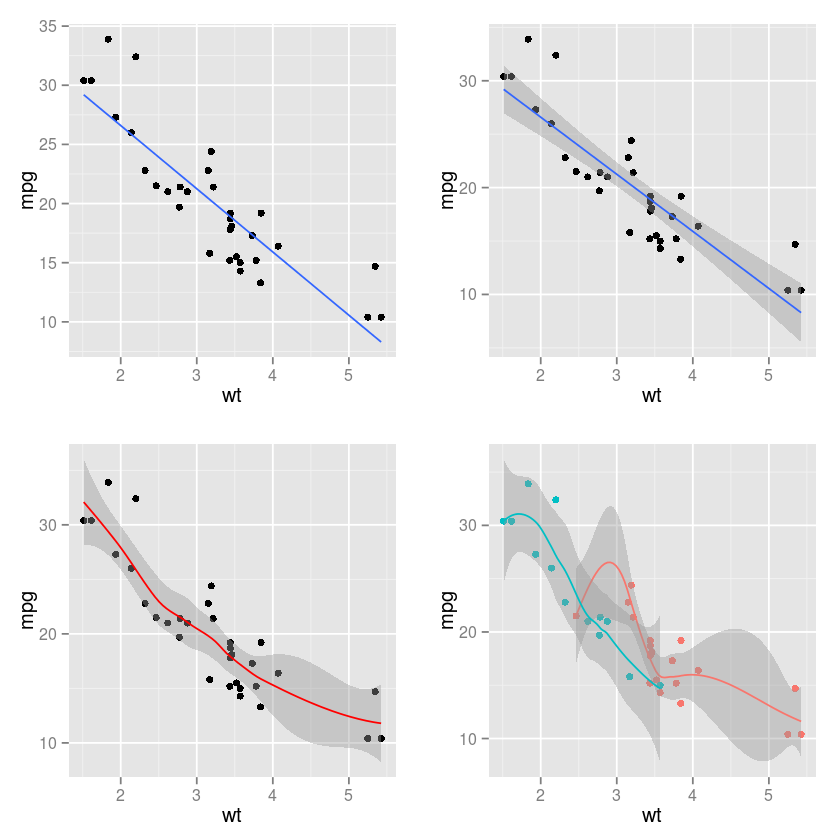
Adding fitted lines¶

p <- ggplot(mtcars, aes(x=wt, y=mpg))
p1 <- p +
      geom_point() +
      stat_smooth(method=lm, se=FALSE)
p2 <- p +
      geom_point() +
      stat_smooth(method=lm, level=0.95)
p3 <- p +
      geom_point() +
      stat_smooth(method=loess, color='red')
p4 <- ggplot(mtcars, aes(x=wt, y=mpg, color=factor(am))) +
      geom_point() +
      geom_smooth(method='loess') +
      guides(color=FALSE)
grid.arrange(p1, p2, p3, p4, ncol = 2)

_images/GGPlot2Graphics_15_0.png

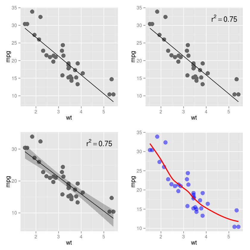
Using existing model fits¶

m1 <- lm(mpg ~ wt, data=mtcars)
pred1 <- data.frame(wt=seq(min(mtcars$wt), max(mtcars$wt), length.out=100))
pred <- predict(m1, pred1, se.fit=TRUE)
pred1$mpg <- pred$fit
pred1$low <- pred1$mpg - 1.96*pred$se.fit
pred1$high <- pred1$mpg + 1.96*pred$se.fit

m2 <- loess(mpg ~ wt, data=mtcars)
pred2 <- data.frame(wt=seq(min(mtcars$wt), max(mtcars$wt), length.out=100))
pred2$mpg <- predict(m2, pred2)

p <- ggplot(mtcars, aes(x=wt, y=mpg))
p1 <- p +
      geom_point(size=4, color='gray40') +
      geom_line(data=pred1)
p2 <- p +
      geom_point(size=4, color='gray40') +
      geom_line(data=pred1) +
      annotate("text", label="r^2 == 0.75", parse=TRUE, x=4.8, y=32)
p3 <- p +
      geom_point(size=4, color='gray40') +
      geom_line(data=pred1) +
      geom_ribbon(data=pred1, aes(ymin=low, ymax=high), alpha=0.3) +
      annotate("text", label="r^2 == 0.75", parse=TRUE, x=4.8, y=32)
p4 <- p +
      geom_point(size=4, color='blue', alpha=0.5) +
      geom_line(data=pred2, color='red', size=1)
grid.arrange(p1, p2, p3, p4, ncol = 2)

_images/GGPlot2Graphics_19_0.png

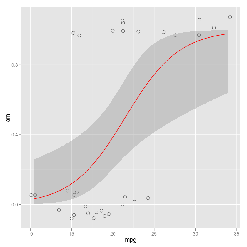
Fitting a lgoistic¶

ggplot(mtcars, aes(x=mpg, y=am)) +
geom_point(position=position_jitter(width=.3, height=.08), shape=21, alpha=0.6, size=3) +
stat_smooth(method=glm, family=binomial, color="red")

_images/GGPlot2Graphics_21_0.png